Land Cover Classification: How It Works At EOSDA

Why Businesses Order Land Cover Classification

If you are new to geospatial analysis, you might be wondering why businesses are increasingly ordering LULC classification. You can look at an RGB satellite image and identify what’s what with your own eyes. Why do they go for color-coded raster images of the forest if they have already seen the forest on RGB?

The answer is – quantitative evaluation. Businesses have to put change dynamics into numbers, otherwise, they won’t be able to manage land usage. They want to predict how much of an end product they can produce and sell based on the crop yield, allocate the necessary budget, and come up with relevant engineering solutions, logistics, etc. Meanwhile, the visual representation of a LULC classification in simple colors on a geographical map helps humans comprehend the information about classification results. Some patterns you can only see when you visualize the data and analyze it from a human’s perspective, throwing into the mix your intuition, individual memories and perceptions, and non-linear logical patterns that even the smartest machine would’ve never guessed.

It is essential to always fine-tune the accuracy of LULC mapping algorithms because the land cover is a highly fluctuating value – it never stays the same. Seasons change, water levels come and go, rains fall, and so on. So, a neural network has to continuously adjust to new circumstances and their connections with one another.

For example, if you are dealing with a spring flood on a flat surface, how do you know where the water goes this time? It’s like spilling a glass of water on a table – the outcome trajectory is overall understandable but a bit uncertain, depending on the texture and size of your table, the speed of turning the glass upside down, the objects on it, etc. Similarly, the flood stream can literally go anywhere, but it does have some dependencies which are nearly impossible to predict with the human brain because there are so many changing variables with different levels of correlation. That’s where AI comes in.

The team of EOSDA scientists continuously works on training neural network models for land cover classification. To maintain the utmost accuracy, we’ve developed a custom fully connected regression model (FCRM). Let’s see how it works and review some prominent examples where our algorithm achieved great results.

Land Cover Classification: How We Do It

1. Collecting and preprocessing the data: First, we gather satellite images and corresponding ground truth data (like weather or precipitation levels) for different land cover classes. We preprocess the data by building a time series for classification, segmenting images into patches, and encoding the ground truth labels.

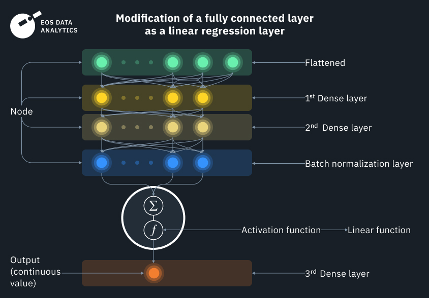
2. Designing the architecture: At this stage, we code a custom fully connected regression model (FCRM) for each class, which is modified into a linear regression on the output. All these terms might sound foreign to you if you haven’t been dealing with neural networks before, but in actuality, they are simpler than they may seem. For example, fully connected means that all inputs and all nodes (layers) have connections with one another, whereas the simplest linear regression can be described as a linear equation in slope-intercept form,

In a neural net, you can think of satellite (input) data as x and y, and the function itself as a neuron. Just like physical neurons, the function neurons only fire if a certain condition is met.

In our algorithm, we have multiple neurons (functions) that are all connected with each other. At the output, we get a linear regression activation function taking multiple logistic (binary) regressions as input, which is a pretty neat solution. The model has to make lots of multivariate choices before deciding on a final result. It’s like an overblown if-condition for every pixel in which a satellite image breaks down, transforms, and then gets itself back together just like BumbleBee.

The continuous output data shows the probability of the initial input belonging to a certain class. So, first, we obtain the multitude of possible values, then divide it into ranges which show a measure of the relation between the input variables. Finally, a certain class is given to a chosen range.

3. Splitting the dataset: We divide the preprocessed dataset into training, validation, and testing sets using an appropriate ratio (e.g., 70% training, 15% validation, and 15% testing). We also try to make sure that all sets have a balanced representation of classes.

4. Training the models: We train each FCRM separately on the training set by minimizing the Mean Squared Error (MSE) between predicted probabilities and ground truth labels. During training, we use optimization algorithms to update model parameters iteratively. Then, we regularize the models to prevent overfitting (learning on noise) by employing techniques like dropout or weight decay.

5. Monitoring validation performance: We track the performance of each FCRM on the validation set during training using evaluation metrics such as R-squared or mean absolute error (MAE). We adjust hyperparameters like learning rate, batch size, or model complexity if we need to optimize performance. There is usually no one-size-fits-all solution when it comes to these parameters, so we fine-tune them every time.

6. Ensemble modeling: We combine predictions from individual FCRMs to obtain a final land cover type classification by employing ensemble methods.

7. Evaluating the test set performance: We assess the overall performance of our algorithm on test data (previously unseen by a model) using metrics like statistical error and confusion matrix.

8. Fine-tuning and iterating: At this stage, we iterate over steps 2-7, refining the architecture, hyperparameters, or ensemble method to improve classification performance.

9. Cropping the final result by the frame: Finally, we are preparing the output visualizations with respect to predefined AOI (area of interest) coordinates.

Difference In Classification: Comparison Between EOSDA And Reference Sources

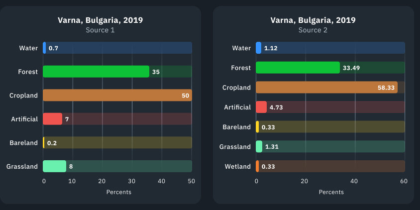
We compared our classification results with the LULC open data provided by two reference sources to validate the output generated by our model. Let’s call them Source 1 and Source 2.

Source 1 offers data from 2017 to 2022, while the Source 2’s data ranges from 2015 to 2019. We noticed that LULC classification results from large companies can vary. One possible reason for these discrepancies in land cover classification is the different class aggregation methods employed. For example, one data provider may classify forests as a single class, whereas another provider’s model distinguishes between sparse and dense forests. Consequently, classes representing relatively small areas within the territory of interest can exhibit significant differences, as shown in the visualization below. However, this does not apply to year-to-year changes within the same class.

On the visualizations and charts, you can see the territory of Varna city, Bulgaria. Usually, the classes do not stay the same, instead fluctuating a bit from year to year. The bar charts below show a more detailed breakdown of 2019 as it is common to both reference sources, also demonstrating differences within 2019.

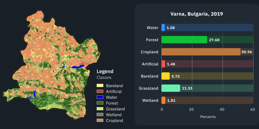
The following visualization and bar chart shows the statistics received from the EOSDA model. As you can see, the classification results are a bit different.

A striking example: EOS Data Analytics LULC classification provides Grassland class for both pasture areas and areas with the presence of undersized shrubs, while Source 2 classification demonstrates these values are in completely different classes. For this reason, the percentage of classes may differ.

After the comparison, we concluded that land cover classification results from different models may vary. This might be due to the fact that objects that appear to be visually alike but different in nature, might be classified as one class or another, depending on the algorithm, input data, training process, etc. To assess the level of accuracy with the highest precision level, we would need to analyze the particular use case and ground truth validation data.

Examples Of Land Cover Classification By EOSDA

As you can see from the comparison above, EOSDA scientists were able to achieve a high level of detail in our LULC algorithm. In essence, the factor that could have contributed the most was the use of short periods of satellite time-series data. This approach also allows us to get a sharpened view of identified classes. Although, we must admit that the input data has to be sufficient, too.

For further validation of our model on various landscapes and climate conditions, we trained it on the data from a few different regions. Take a look at the examples below to see the training results.

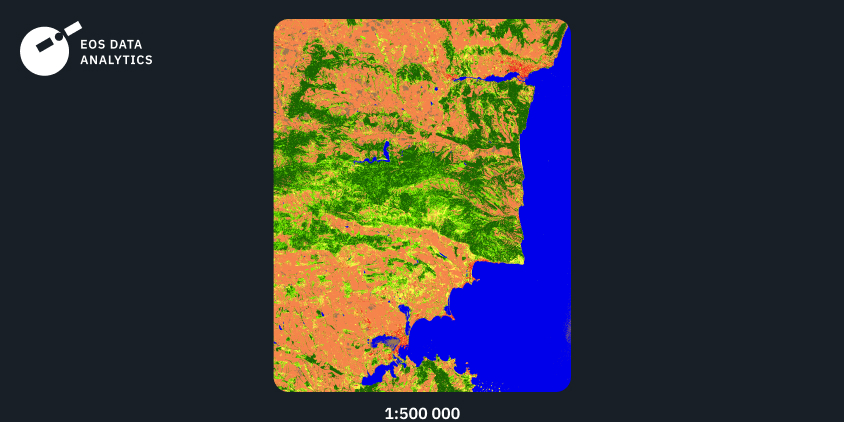
Region №1: Bulgaria, 2021

Let’s close up on the LULC classification results obtained by the EOS Data Analytics model in Bulgaria. Here we can see a very precise identification of forest, water, and cropland classes. It’s worth mentioning that the latter has tight dependencies between the number of obtained input images, seasonal fluctuations, and the output result.

As we can tell from the output result, the EOSDA scientists trained the model on a sufficient number and quality of input data. The yellow-colored bareland class includes a detailed fixation of the local pavement infrastructure. The model also identified artificial objects.

Region №2: Nigeria, 2021

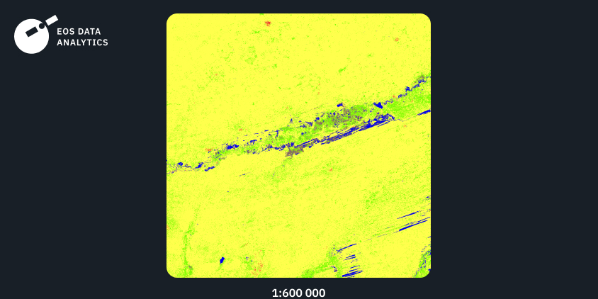
This training output shows that the model identified dry lands of Nigeria as a bareland class. Nevertheless, a small amount of water and grassland is also identified with precise detalization. Even smaller territories of a wetland class show seasonal flood (or a lack thereof, which might signify a drought).

Region №3: South America, 2021

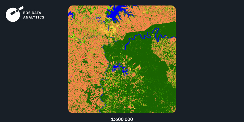
The third example shows the output of our model trained on the input data from South America. Again, we can see a high level of detail combined with smooth transitions between the classes. While the forest class is predominant in the given AOI, the grassland class is precisely distinguished from the forest class.

Closing Thoughts

Businesses across multiple domains can leverage our models to gain deeper insights into land usage patterns, optimize resource allocation, and make informed decisions to increase profitability. From a greater perspective, by obtaining an inch-by-inch land cover classification of the territories of interest, communities can take necessary action to save the environment and build sustainable infrastructures.

Every custom-trained model at EOSDA is based on an algorithm supervised by humans, that’s why we are able to achieve such a striking quality of the output results. As a starting point, we’ve already trained our LULC model on different geographies’ data, as you can see in this article. By further refining architecture and data parameters in every given case iteratively, our scientists are able to achieve significantly lower statistical error, i.e. increase the accuracy of classification.

Another benefit is that the more custom LULC models our scientists supervise, the more context they have at hand. As a result, they can build smarter models than someone with no experience in this field. We are continuously gaining valuable insights into how satellite monitoring contributes to the efficient management of land resources, along with environmental conservation efforts and climate change research.