Time series analysis of satellite images is a valuable tool for investigating the dynamic processes at work on our planet. We may get insight into many different fields, from farming and forestry to city planning, by collecting and analyzing images captured over time. This article delves into the practical uses of time series satellite data and how it is currently shaping managerial decisions. Experts from all fields can benefit from satellite imagery time series by gaining a deeper understanding of complex events, designing more effective strategies for managing resources, and laying the groundwork for sustainable development.
Satellite Imagery Time Series: What Is It And Why Use It?
A satellite imagery time series is a sequence of images (data points) of the same location recorded at regular intervals throughout a given period of study. Here, time is a critical factor that adds depth to the available satellite data because it reveals not only the end results but also the changes during the span of the data points.
Time series analysis is a common use of the information gathered. It typically calls for many satellite observations to ensure data validity, precision, and consistency. Working with large data sets provides the option of eliminating random effects and correcting for seasonal swings. Meanwhile, detecting trends and seasonal changes in satellite image time series gives additional information useful for making more educated decisions. Real-world applications of time-series satellite remote sensing data include using past events as a basis for making predictions about the future.
Let’s say at the start of the growing season you plan to build a time series graph based on historical satellite images. It comes as a shock to learn that one of your fields is producing significantly less compared to the same period in past years. The key to preventing future devastating crop failures is identifying the issue as soon as possible so that its source may be isolated and eradicated. Long-term analysis of time series of satellite images can sort out tons of data collected over several years, apply the appropriate vegetation indices to each image, and help you spot trends in this mountain of data.
By continuously amassing and monitoring live satellite images of the Earth, you may quickly and accurately assess changes, recognize trends and patterns, spot anomalies, and both make sound business decisions and take corrective action in your areas of interest (AOI).
Application Areas For Satellite Data Time Series
Time series of satellite images provide invaluable information for numerous applications. The common thread across these uses is the notion that satellite data can help us learn more about the ways in which the planet is changing, the forces behind these changes, and their potential repercussions.
Agriculture
Farmers can greatly benefit from using time series of satellite images as a source of valuable information about the dynamics of growth and yield of their crops, as well as a helping hand in predicting crop production and agricultural market pricing. In order to prevent economic losses caused by insect infestations, satellite image time series are used for pest and crop health monitoring. Knowing the history of their crops’ vegetation, farmers can optimize the allocation of inputs (water, nutrients, chemicals, seeds, and more) and improve their farm management activities’ planning. Crop monitoring, crop rotation planning, irrigation and fertilizer control, pest and disease management, yield prediction, and land use management are just a few of the many agricultural uses for satellite data time series analysis.
Forestry
The public release of the Landsat data archive, which is known as the most utilized data set for satellite imagery time series analysis, lowered the barrier to entry for forest monitoring . The past decade has also seen additional advancements in forest change detection technology, allowing for greater in-depth monitoring of forests.
The satellite data series can aid in locating problem areas and guide decision-making by observing changes in the state and area of forest cover, overall forest health and composition over time. In particular, by analyzing the time series of satellite images, forestry managers can identify deforestation hotspots and measure the rate at which trees are being cut down. Satellite data series analysis can thereby inform afforestation, reforestation, forest restoration, and other forest management strategies.
Climate Change Monitoring
Satellite imagery time series, the backbone of statistical climate analysis, can yield actionable insights for climate study and policymaking. Climate system computer models based on series of satellite images can be used to monitor Earth’s radiation budget, examine the effects of climate change on plant life, keep tabs on the sea level, observe the shifting of glaciers and ice caps, and much more. As an example, the GEOS-5 Atmosphere-Ocean General Circulation Model (AOGCM) is a state-of-the-art model that seeks to reflect climate variability across many timeframes (from synoptic to multi-century) .
Disaster Management
Time series analysis has many applications in emergency management, including heads-up detection and disaster risk forecasting. Satellite imagery time series also help assess the devastation caused by natural disasters such as earthquakes, storms, floods, landslides, and wildfires (more in our natural disasters 2023 article). With the assistance of this data, disaster management directors may better coordinate response efforts and more efficiently distribute available resources, as well as keep updated on the progress of damaged areas’ restorations.
Land Use Planning
Satellite imagery time series analysis can shed light on land use change and the spread of cities. Such knowledge is essential in the context of sustainable soil use, where the appropriate configuration of various uses (agriculture, forestry, cities, etc.) ensures long-term soil conservation and eco-system balance. Planning and management using time series of satellite images can improve urban buildout, infrastructure, and municipal services. In addition, satellite imagery helps track and analyze the effectiveness of urban transportation systems.
This is merely a small sample of the many real-world applications for satellite imagery time series. Further, the use of satellite data to gain insight into and take action on global concerns will grow exponentially as technology advances.
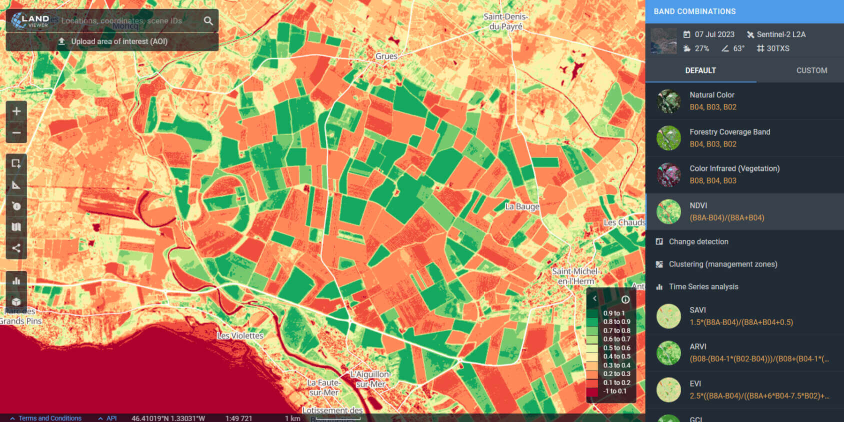
How To Make The Most Of EOSDA LandViewer’s Time Series Feature
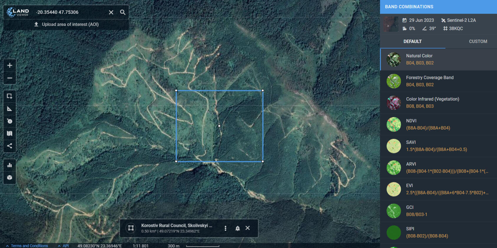
Quickly find and analyze a required time series of satellite images by narrowing in on a specific area of interest with the help of EOSDA LandViewer. Simply define (draw or upload) your AOI, then use the Time Series Analysis function, and the tool will handle the rest.
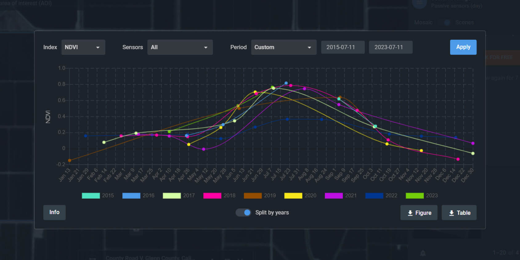
The tool offers three indices to choose from: NDVI, NDWI, and NDSI, and they each serve specific purposes. When a drawdown of any index shows up on the graph, you can visualize the corresponding plot on the map and dive deeper into the analytics to determine what caused the drop.
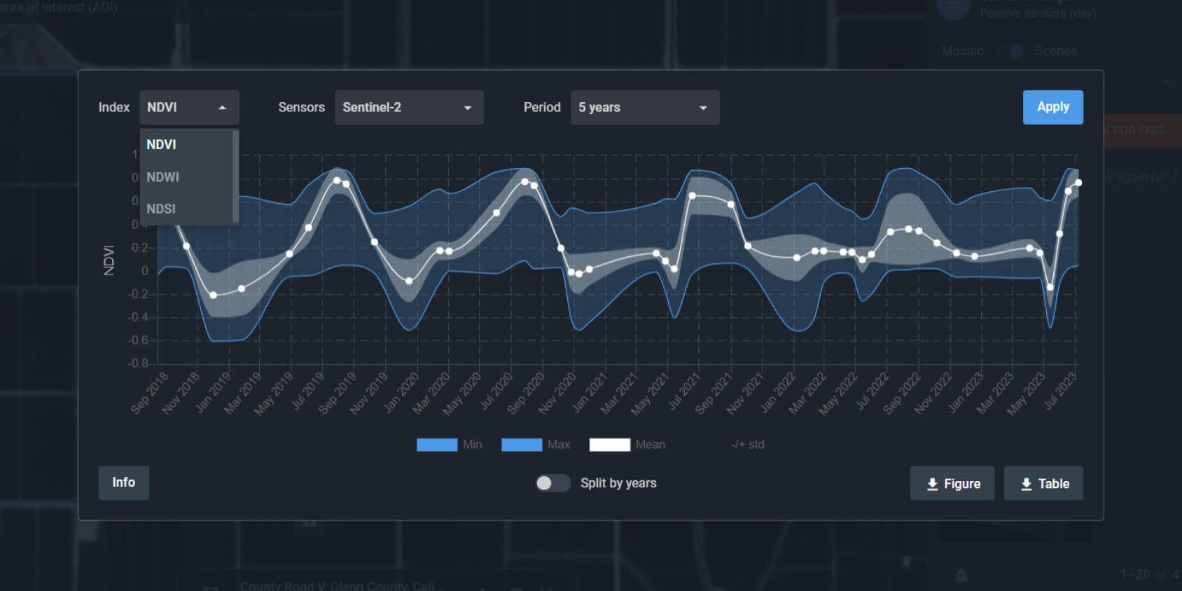
By default, you can generate index graphs covering any interval between one month and ten years. If these ranges do not work for you, you can enter your own using the calendar. The cherry on top is that you may use all of the sensors at once to construct the satellite imagery time series graphs, in addition to choosing the spectral index, the period, and the data source.
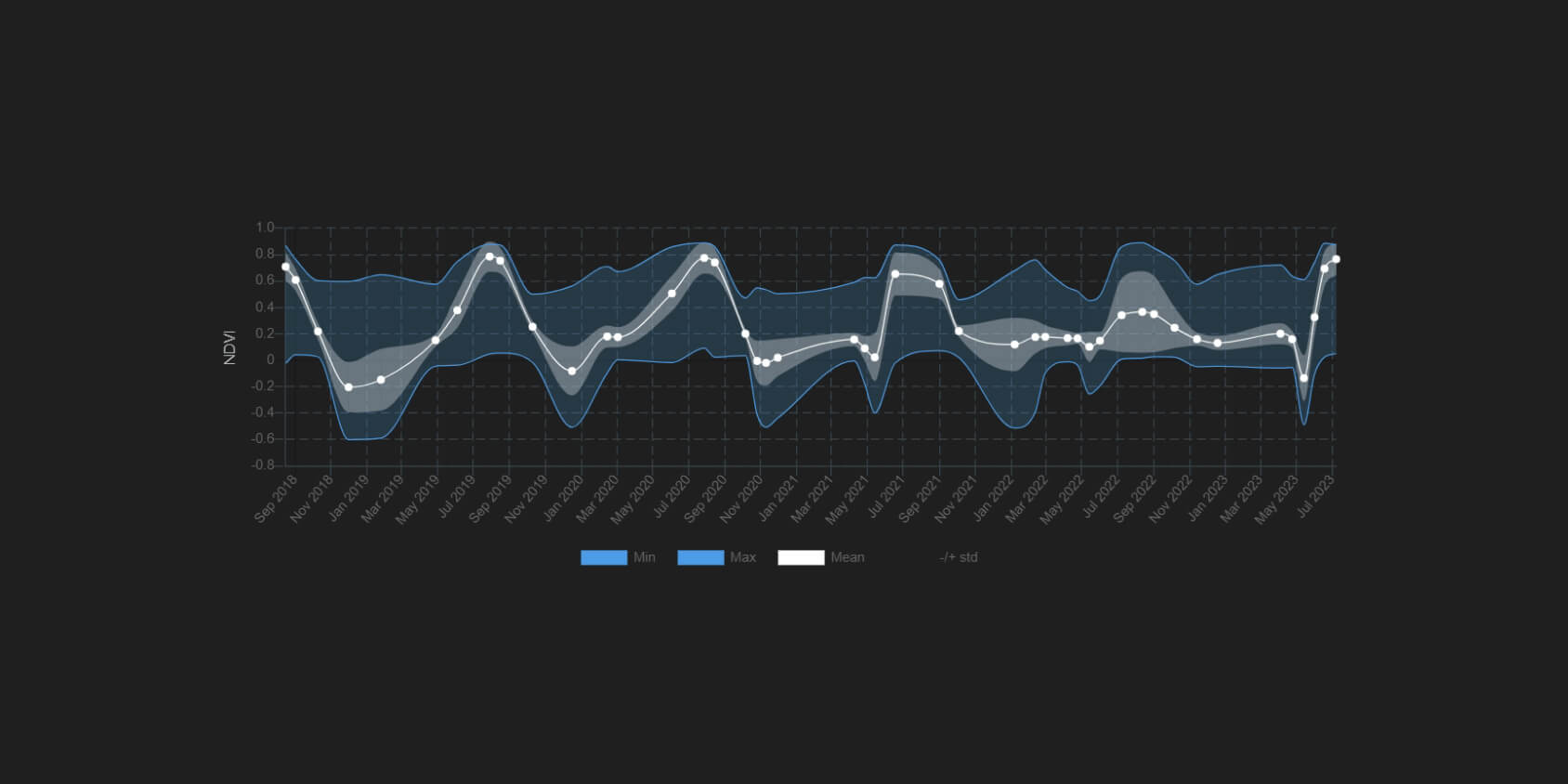
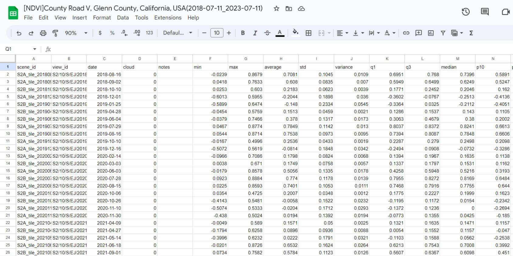
You can compare a field’s performance during the same period in different years with the Splitting by years option. The curve is broken down by year, making it simple to see how the index has changed over the past three to ten years. Check if the values are within the typical ranges by comparing them to what you’ve seen in the past. With the refined representation of satellite imagery Time Series Analysis, you will never again fail to notice a trend or anomaly. For your convenience, both a graphical (in png format) and a tabular representation of the results (in CSV format) are available for download.
Time Series Of Satellite Images In Practice
A time series of satellite images can be a powerful tool for monitoring and managing agricultural and forest land. They provide a wealth of information about changes in vegetation and land use over time. Below, we’ll dive deeper into how satellite imagery time series can be used in the real world.
Monitoring Illegal Deforestation
According to the UN, the Carpathian region is at grave risk due to illegal logging, which necessitates constant monitoring of deforestation and proactive conservation efforts . Let’s do some investigating on our own. Find a location on the map where deforestation’s effects may be seen with the naked eye, and center the AOI there.
With the help of the Time Series Analysis tool, create the NDVI vegetation index graph. Using the index and its accompanying graph, you may determine when biomass levels in the area dropped sharply during a given period. Turning off the smooth curves that don’t show any drawdowns, we can identify the exact year of the largest drop. Select both this year and the next one to plot on the graph.
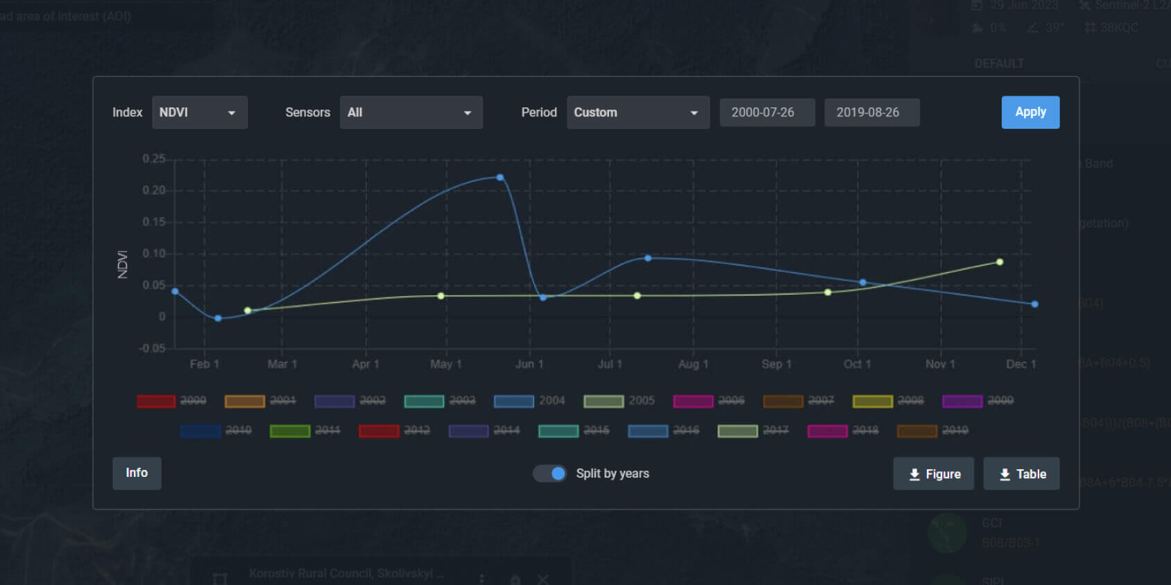
According to the graph, the amount of biomass decreased dramatically in 2004, was low for virtually the entire year of 2005, and then increased towards the end of the year. This increase was due to the wild growth in the previously cut and tramped area of the forest. As you can see, this satellite data analysis took just a few simple steps. You can use what you’ve learned here to quickly and easily find out where and when illegal logging occurred.
Identifying Patterns And Abnormalities In Crop State In A Certain Field
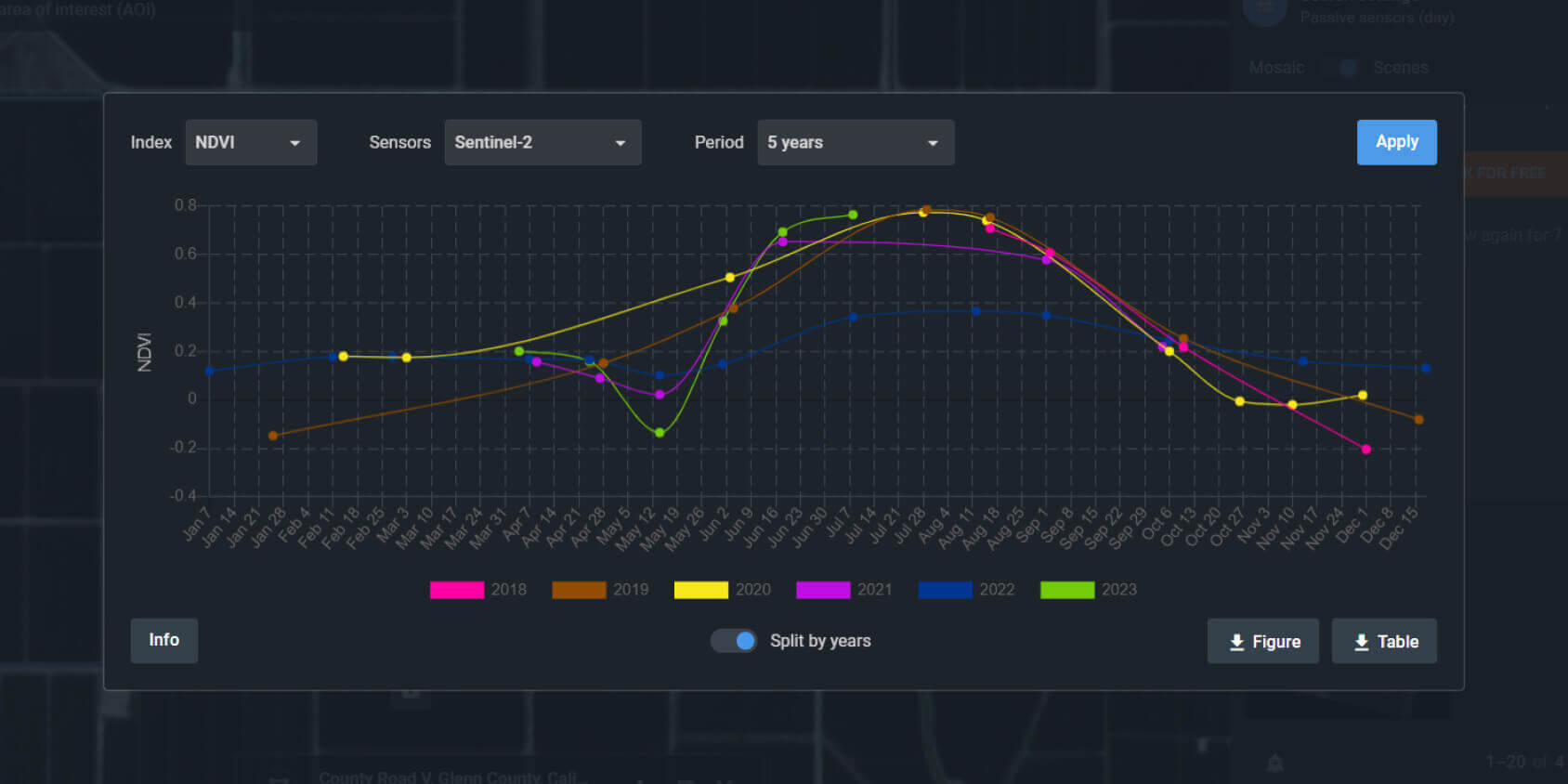
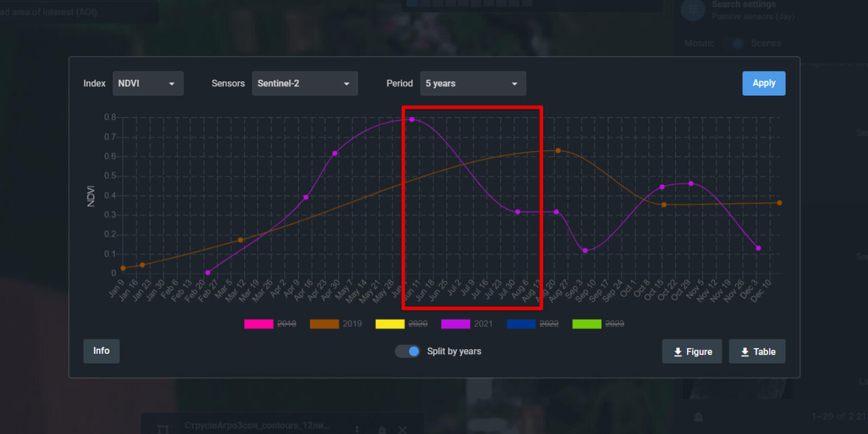
Now, let’s check out the scenario for creating field-specific satellite imagery time series. Take a look at the sequence of years during which the same crop was grown in the field. Using NDVI, we can determine certain trends in the development of this crop.
We’ll focus on the years 2019 and 2021. The record crop in 2019 will serve as a benchmark for future harvests. The gauge of the increase in vegetation is clearly visible from February to August. This is due to the emergence of shoots and active crop growth during this period. The NDVI was also rising steeply from February to the middle of June 2021, though there was a significant decrease after that. Abnormally high temperatures are the reason for this NDVI drop.
So, what does this all boil down to? If you compare the growth of a crop from year to year, you may quickly spot any discrepancies. As we see in the graph, the farmer was able to find the source of the problem and fix it using Time Series Analysis and a comparison of the present NDVI to those of years with high yields.
Determining How Far Field Performance Deviates From Regional Norms
In the next scenario, we’ll take into account not only your fields but also adjacent ones. Let’s use satellite NDVI maps for field monitoring. With their help, we can locate areas of the field where individual plots have widely varying NDVI values.
The question is how to determine if these numbers are the norm or an outlier. And how significant are these differences, if they indeed exist? To answer these questions, we can use the satellite imagery Time Series Analysis tool.
Let’s take other fields within our district and create graphs of their performance for the last three months. From this, we can draw some trends in the development of fields for the whole district. Since many local factors, such as the weather, have an impact on these trends and are relatively constant for such small areas, it is crucial to take the above steps precisely in your region. Once you have created graphs within your region, you can save them as a table to easily compare the performance of one field with others and tell if your fields’ NDVI performance is typical or drastically different from the usual across the entire region.
Improving Your Everyday Decision-Making With Time Series Of Satellite Data
Satellite imagery time series analysis is emerging as a powerful tool for monitoring and understanding Earth’s dynamic processes. Unlike individual satellite photos, which only capture one moment, time series satellite data enables the study of trends and shifts over different periods. Time is an essential variable for researchers examining phenomena as diverse as deforestation, agriculture, climate change, natural disasters, changes in land cover, and urbanization.
Thanks to advances in Earth observation satellites with high-resolution imaging capabilities and more satellite constellations offering higher revisit rates, researchers and decision-makers now have access to an unprecedented amount of data. Artificial intelligence and machine learning algorithms have also helped speed up the examination of huge satellite data sets.
Today, you have the unique opportunity to perform ongoing monitoring of your area of interest with EOSDA LandViewer, a smart tool that combines the advantages of satellites and AI, allowing you to accumulate diverse data and make its subsequent analysis much more precise. You can easily spot patterns, trends, and outliers in your chosen areas by incorporating this satellite imagery time series software into your routine. Email us at sales@eosda.com if you’re interested in learning more about the Time Series Analysis feature and how it may help you address everyday challenges and shape a sustainable future through data-driven decisions.
About the author:
Petro Kogut has a PhD in Physics and Mathematics and is the author of multiple scientific publications. He is the Soros Associated Professor as well as the head of the department of differential equations in the Oles Honchar Dnipro National University and has received a number of grants, prizes, honorary decorations, medals, and other awards. Prof. Dr. Petro Kogut is a science advisor for EOSDA.

More news
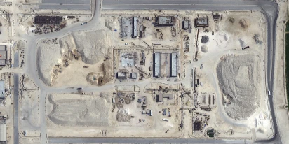
Construction site monitoring: The guide to remote progress tracking with satellite images
From cameras and drones to satellites: a practical look at how construction site monitoring works, where each tool shines, and what a remote, orbital view actually adds.
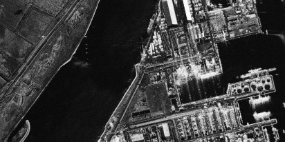
SAR imagery: How synthetic aperture radar technology works
Want to monitor assets without weather delays? Learn how SAR imagery captures soil moisture, floods, and structural shifts through clouds and smoke for your monitoring projects.

Optical satellite imagery: Getting insights from space
Ground inspections can be slow and expensive. Discover how commercial optical satellite imagery simplifies remote site monitoring and supports daily operational decisions.