EOSDA Custom Neural Net: Deforestation Detection
When thinking about industries that are associated with rising levels of CO2 emissions, sectors that are “closer to nature” are the last thing that comes to mind. However, research shows that forestry and agriculture are responsible for more than 5.3 Gt of CO2 emitted annually due to deforestation, which makes these industries the second largest source of anthropogenic carbon emission. What’s more, tree felling in tropical forests also reduces the amount of soil organic carbon and endangers biodiversity . Regulatory bodies at a global scale have already taken action regarding this issue. For example, the EU will restrict market availability and export of products that are associated with deforestation activities .
To stay compliant with international regulations and contribute to environment conservation, it’s crucial to implement means for accurate deforestation detection.
EOS Data Analytics is dedicated to providing space solutions for Earth’s problems. By leveraging GIS data and custom AI algorithms, we strive to preserve the environment we live in. With our expertise in remote sensing and data analysis, we decided to contribute to deforestation detection efforts in the EU by monitoring forest cover changes, identifying illegal logging activities, and supporting conservation initiatives by delivering accurate and timely information.
Our Science team has developed a deep-learning neural network algorithm based on the methodology described in Mapping Tropical Forest Cover and Deforestation with Planet NICFI Satellite Images and Deep Learning in Mato Grosso State (Brazil) from 2015 to 2021 . In this blog post, we are giving a high-level overview of how it works.
The Process Of Creating The Deforestation Detection AI
The decision-making process within computer vision models, which enables them to differentiate between distinct object classes, is highly complex.
EOS Data Analytics is proud to represent the expertise of 60 data scientists including 25 PhDs. To get started with creating a deforestation detection model, our teams of AI and GIS scientists elicited functional requirements. They concluded that the model should:
- Recognize and filter out the noise (clouds and other visual distortions)
- Identify change dynamics of deforestation (true positives, true negatives)
- Identify falsely identified forest/non-forest classes (false positives, false negatives) and run algorithms to determine and assign true values.
To meet these requirements, we had to carefully evaluate our choices regarding source imagery, architectural design, and innovative solutions to address novel algorithmic challenges.
Imagery
Before diving into the intricacies of algorithms, we needed to obtain high-quality satellite imagery datasets to work with.
For the purpose of this research, we have chosen PlanetScope. This source provides mosaics that represent an average best image from multiple ones taken during the month. As a result, they generally include fewer clouds which makes this imagery fairly consistent for efficient training of classification models. Later on, we also experimented with different kinds of channels, tiles, architectures (UNet & MobileNet), and imagery samples, which allowed us to construct an optimal custom neural net. Below, we demonstrate some of the stages of our successful experiments. While the described routine doesn’t represent the entire complexity of the process, it highlights some key findings that showed to be efficient, transferable, and valuable for our future deforestation detection products and services.
Architecture
To conduct the initial segmentation of the area of interest, we used U-Net architecture. It takes raw images and gives a complete segmentation as the output, leveraging the series of convolutional neural networks within itself to study the image features. This type of architecture uses the encoder-decoder logic, shrinking down the images, finding patterns, and then expanding them back, which is why the learning phase looks like a letter “U” .
In our case, the model received a 4-band image (Fig. 1). We found that it benefits from assessing the visible light spectrum complemented by the near-infrared, which is one of the interesting approaches that we found in a series of experiments. At the output, we have a binary mask, where each pixel corresponds to either 0 (not a forest) or 1 (forest).
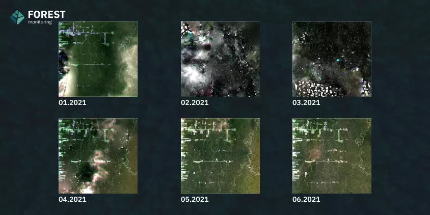
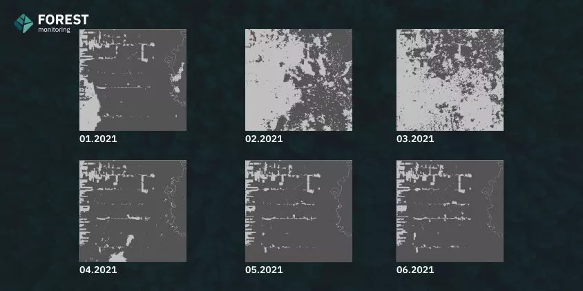
As you can see in the images above, clouds and noise are classified as non-forest (Fig. 2). In our next step, we will run an algorithm that filters out the clouds from these initial segmentation results.
On the one hand, we do want clouds to be classified as non-forest. Since these are binary masks, it would’ve been worse if they were classified as forest. On the other hand, we don’t know what is beneath the clouds so we cannot track deforestation. That’s why we trained the model to first recognize clouds only to apply the cloud filter that would get rid of the clouds. After that, we were able to train an additional model to distinguish trees from bushes, roads, bare land, and more.
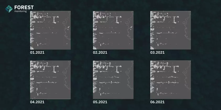
After applying this filter, the output looks much cleaner (Fig. 3). That is because the algorithm assigns a forest value to a pixel only if the forest was detected in at least half of the observations in the specified period. The latter was carefully chosen by our team after a series of additional experiments. Eventually, we found the ideal satellite time series range before and after the specified date. Cloud filter essentially refers to those additional images (when there were supposedly no clouds) to recreate the accurate land cover of the questionable area.
Confidence Scale
At this point, we’ve got clean forest and non-forest binary masks that we will apply in the model’s final deforestation classification process (Fig. 4-6).
Next, we analyze the semi-annual time series and construct a map of felling and forest cover over that period of time. To do that, we calculate the confidence scale (how confident the model is that this pixel belongs to a certain class – forest/non-forest/felling) according to the following rules:
| Confidence score | Status | Description |
|---|---|---|
| 1 | Confirmed | Same class on all 6 masks, e.g., felling, results in felling confirmed |
| 2 | High Confidence (Most Likely) | Same class, e.g. forest is observed for almost the entire period but is not a forest for one or two dates, and these dates are not the first and last dates of the period. For example, if a pixel is a forest from January to June, but in May, the model detects it as non-forest due to clouds, then we assign this pixel a forest class with high confidence. |
| 3 | Unconfirmed | Applies only to felling for the latest date, which cannot be confirmed. A felling is unconfirmed when on date N – 1 we had forest, on date N – no forest, and we have no data for date N + 1 to confirm or deny this felling. |
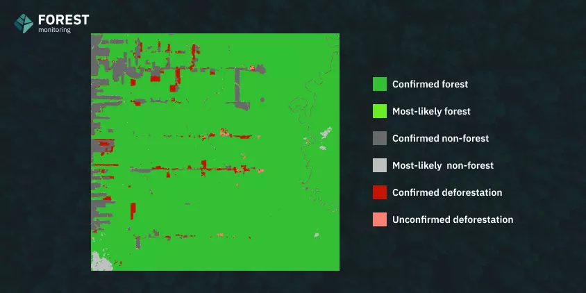
Output Data:
- Deforestation map, including three classes: forest, non-forest, and felling
- Confidence Scale, including three scores: result confirmed, high confidence, not confirmed
Here, forest and non-forest classes can have only two statuses – confirmed and most likely. Similarly, a felling class can also have only two statuses – confirmed and unconfirmed. Thus, we can estimate how the forest cover changed in six months by analyzing one binary mask after another from the present to the past, thereby registering the change dynamics.
EOSDA’s Proprietary Cloud Correction For Residual Uncertainties
Although we’ve gotten rid of clouds before, some of them may still be present on semi-annual felling and forest cover maps. We have developed two additional correction algorithms that apply to semi-annual maps.
The decisions they make depend on the model’s observations:
- Deforest before + forest after = forest before
- Non-forest before + forest after = forest before
Just like with the confidence scale that we mentioned above, here we can’t confirm the latest dates because we have no data to verify these results.
However, there’s an interesting approach that we can apply if we go back in time. We can verify older maps with previously verified newer maps. For example, a map for December 2022 verifies a map for June 2022, which in turn verifies an even earlier map for December 2021. By doing that, we can retrospectively assess deforestation dynamics over multiple years.
Results Of Training
In the examples below, we used 11 distinct masks for each date throughout our periods of interest. Such methodological choice aimed to optimize the model’s accuracy in classification while reducing potential errors.
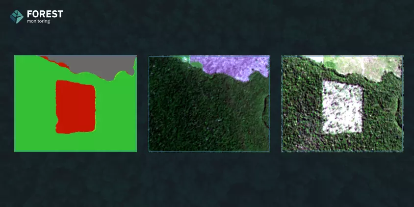
With semi-annual maps of felling and forest cover, we can track deforestation over time and create monitoring maps. Such maps allow us to track deforestation volumes over a period of time and compare deforestation rates, trends, etc. In this example above, we created a two-year monitoring map using four semi-annual masks. We can also create such maps for longer periods of time, provided that we have the required imagery.
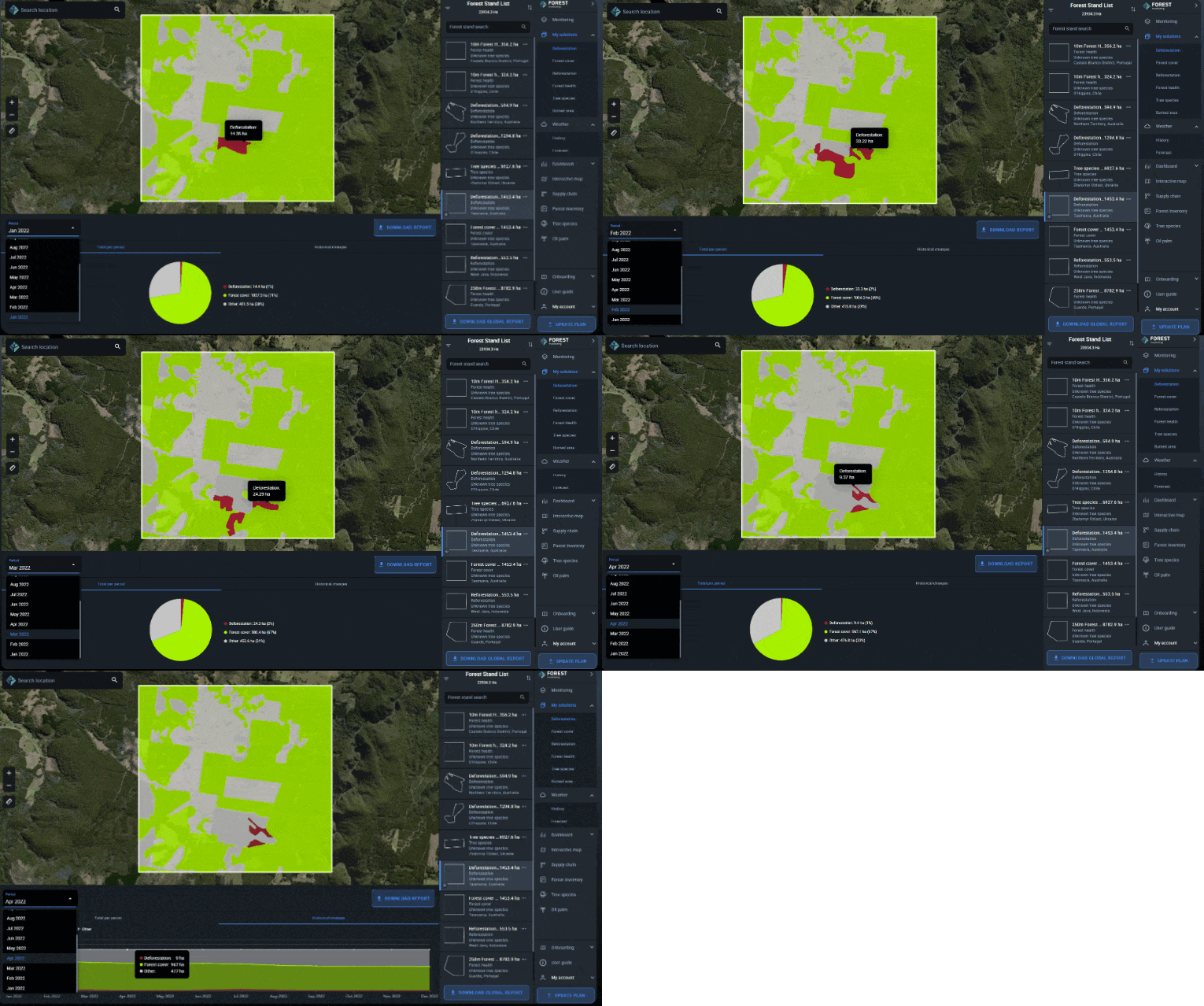
These custom solutions can either be sent in reports directly to stakeholders or be implemented within the web interface of EOSDA Forest Monitoring, which is especially relevant given that the new EUDR (European Union’s Deforestation-free Regulation) comes into force by the end of 2024.
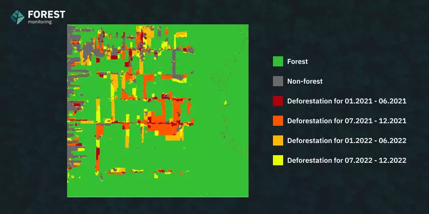
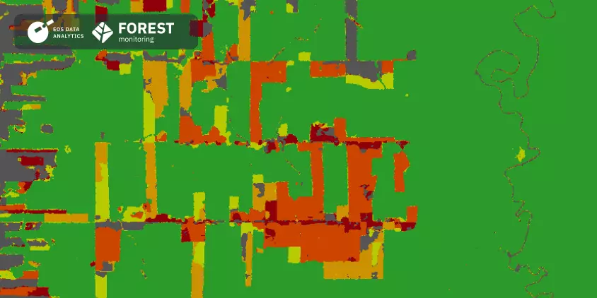
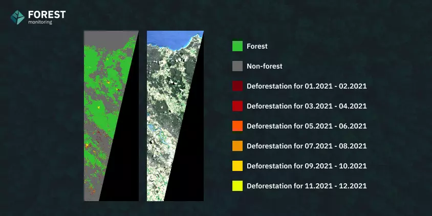
The value of deforestation detection models is especially evident when we zoom out and consider tracking large areas. Take a look at the example below (Fig. 7). In this case, tracking the presence or disappearance of trees seems like a humanly impossible task. Meanwhile, it is achievable and has been automated with our machine-learning model.
Availability Of Custom Deforestation Models In The Future
After experimenting with a variety of satellite imagery types, neural net architectures, and algorithms, we found an optimal combination that allows us to continuously detect tree felling with a high degree of confidence.
From a long-term perspective, it is possible to build both retrospective deforestation maps for certain time periods and monitoring maps to assess the rate and volume of deforestation as time goes by. This model can work as part of user-facing applications.
Forest areas are very large, especially in tropical regions. It is virtually impossible to have a big enough team of GIS specialists to look at satellite images and monitor such areas in an attempt to continuously track deforestation. We created this model to simplify this process, providing opportunities to derive data-driven insights. Upon implementation, users will effortlessly monitor the rate, pace, and patterns of deforestation taking place in their area of interest.
Our novel algorithm presents a new and alternative approach for deforestation monitoring, effectively mitigating erroneous predictions linked to various sources of interference, including cloud cover and imperfections in image quality. The outcomes were corroborated using Sentinel-2 images, affirming the neural network’s accurate detection capabilities. These images encompass spatial resolutions and scene partitions that are different from Planet, therefore enhancing the algorithm’s versatility. The resulting neural network architecture is adapted to the use of Sentinel-2 and EOS SAT-1 imagery.
The resulting quality of any machine learning method is very much dependent on the input data, so further evolution of our model can be achieved by utilizing images that don’t require much filtering and false positives/negatives correction.
Considering these factors, exploring alternative sources like the EOS SAT-1 satellite, developed for EOS Data Analytics, presents an opportunity to enhance the input data for more precise and detailed outcomes, given its impressive 1.5-meter per pixel resolution.
About the author:
Karolina is currently pursuing a BSc at Pennsylvania State University. She excels in communicating the scientific value of EOSDA precision and sustainable solutions in an easy-to-read way. Karolina is a dedicated advocate for personal empowerment striving to represent and uplift Ukrainian women in the global STEM community. She’s a member of AWIS, WIT and other organizations.
Recent articles
EOSDA to Monitor Wildfires in Portugal Using Satellite Data Under ESA’s InCubed Programme
The company signed a contract with ESA to create an innovative satellite-based solution for forest monitoring and wildfire prevention.
EOSDA Forecasts Yields For 2025 In Saskatchewan
EOSDA created RM-level crop yield forecasts for Saskatchewan to address limitations of official data. The project shows how satellite and weather inputs reveal local yield changes during the season.
Digital Tools Improve Soil Health And Yields In Mexico
EOSDA and ITTA supported a Guanajuato farm with contour-line planning, monitoring tools, and practical guidance to reduce soil erosion and improve yields in the long run.