EOSDA LandViewer Guide Search

Introduction to my EOSDA LandViewer

Welcome to EOSDA LandViewer – your online GIS-assistant!

EOSDA LandViewer features overview

1. Integrated into EOSDA Platform, EOSDA LandViewer helps complete the following tasks:

• pick the image from the largest satellite imagery catalog
• instantly process and analyze it with the set of advanced tools
• save, download and integrate spatial data in multiple formats

2. The leading features of the instrument are:

• search by AOI
• advanced satellite filters 
• on-the-fly processing
• custom indices/band combinations
• time series analysis
• time lapse
• clustering
• adding data to the WMS layer
• share and publish

3. The USP of the instrument is:

• instant access to web satellite data
• mosaic approach
• online processing
• high-resolution images (preview and purchasing)
• scene downloading 
• integration with both EOSDA Platform and 3-d party GIS software

Integration with EOSDA Platform

EOSDA LandViewer is a part of an ecosystem of four mutually integrated EOSDA products:

• EOSDA Storage is developed to store, share, distribute and get instant access to thousands of Terabytes of Earth Observation and GIS related data.
• Aspectum is employed to visualize data sets; it creates data-driven maps with SQL-based interface and state-of-the-art cartographic tools.

The instrument allows making a full circle of geodata workflow in one suit. Search, process on-the-fly and pick an appropriate image from the largest satellite imagery catalogue in EOSDA LandViewer, save it to your personal (256Gb) cloud and get the instant access, share and distribute your big data in EOSDA Storage and perform efficient analysis via visualization and SQL-based approach in Aspectum.

Sign Up

To sign up for EOSDA LandViewer, please follow some simple steps:

1. Go to EOSDA LandViewer page

2.  Click Sign up and enter all the required credentials. Note, you are also able to log in with G+, LinkedIn or Facebook account

3. In case, you have already signed up for one of the EOSDA Platform products, click Sign in and enter your login (e-mail) and password

4. Welcome to EOSDA LandViewer!

Find Location

To get started with EOSDA LandViewer, you need to find the Location first. There are several ways to fulfil the task:

• enter the address in the Search box

• enter coordinates in the Search box

• enter scene ID (https://www.usgs.gov/land-resources/nli/landsat/landsat-collections) in the Search box

• scroll around, find the location on the map and stick it with a pointer

AOI (Area of Interest)

Once the Location is found, LV marks it with polygon by default. You can also specify the area that better fits your interest, using AOI  – an instrument for working with a specific area of image. To set the AOI in EOSDA LandViewer, select one of the following options:

• draw the “rectangular AOI”, using the tool-box in the left sidebar

• draw the “circular AOI”

• draw the “polygonal AOI”. The polygon tool allows you to add points and outline your AOI as precise as possible

• upload your KML, GeoJSON, Shp file in EOSDA LandViewer. Once you click AOI icon, the tabs My AOI (the list of the saved AOI’s) and My Subscriptions (the list of AOI’s you are subscribed for) show up in the menu on the left

• in the bottom of the main menu click Upload AOI and select the necessary file

• Once the file is uploaded, add it to the list of AOI’s, clicking Save button below the selected AOI or in the context menu in the bottom centre of the screen

• download AOI in .geojson/.kml/.shp formats

Customize AOI

Use the Сontext menu to customize your AOI, that is:

• hide the AOI

• select the area units: kilometers or miles

• convert it to measurements to check the Distance and Area of your AOI. Click the icon once again to discard changes

Subscribe to My AOI

My AOI allows you to draw your target area, save it to My AOI list and use it across all the EOSDA Platform products. To Subscribe to MY AOI and get notifications about the newest satellite images of the saved area:

• select the AOI; once AOI is set, the list of images from all the satellites available in EOSDA LandViewer shows up in the right sidebar.

• hover over the images, one by one, to choose the one that covers your AOI entirely

• apply the filters and select the Scene that fits your AOI most

• click the “bell” icon under the list of the images and confirm your subscription

• check the AOI details and click Subscribe to get email notifications every time new satellite images are added

Satellite filters

Once the AOI is set, take the following steps to choose the image that fits your AOI most:

1. Click All Filters and select the Source from the drop-down menu:

• passive sensors (day) -Sentinel-2 L1C, Landsat 8 OLI + TIRS, Landsat 7 ETM +, Landsat 4-5 TM, Landsat 4-5 MSS, CBERS 4 MUX, CBERS 4 WFI, CBERS 4 PAN 10, CBERS 4 PAN5, NAIP.
• passive sensors (night) –  Landsat 8 OLI + TIRS, Landsat 7 ETM+, Landsat 4-5 TM.
• passive sensors (low resolution) – MODIS MCD43A4
• active sensors – Sentinel-1 GRD IW,  Sentinel-1 GRD EW, Sentinel-1 GRD SM
• terrain Tiles
• high-resolution images – SPOT 5, SPOT 6,7 Pleiades 1A, 1B, KOMPSAT-2, KOMPSAT-3, KOMPSAT 3-A, SuperView, Gaofen 1, Gaofen 2, Ziyuan-3, TripleSat
• EOSDA Storage files – all the files, saved in EOSDA Storage

2. Once the Source, in this case Passive sensors (day) is selected, you can either unclick the satellites you don’t need from the All sensors list, which shows up by default once the Source is chosen, or hover over the necessary satellite, select Only and all the other satellites will be excluded from the list automatically

3. Hover over the satellite image to check if it covers your AOI entirely

4. Check the image details – date, source data, sun elevation, cloudiness, the orbital path number as well as polarisation and shooting mode, in case of radar sensing,  in the right side of the image

5. Set the Date or Date period, selecting the start date and the end date

6. Set Сloudiness and Sun Elevation. The cloudiness value (0-100%) is set to 100% by default. The Sun Elevation (0-90°, with min. value=1) is set to 90°

7. Set Polarisation in active sensors dataset

Polarisation can be one of  SH (single HH polarisation), SV (single VV polarisation), DH (dual HH+HV polarisation) and DV (dual VV+VH polarisation)

The active sensor images are available in IW (The Interferometric Wide) swath mode – the main acquisition mode over land, which satisfies the majority of service requirements. It acquires data with a 250 km swath at 5 m by 20 m spatial resolution

Band combination

Using Band Combination tab select specific bands from a multispectral satellite image to create color pictures that are specifically tailored to facilitate the identification of the features of interest. Choose any of the following ways to use it:

• Click the Band combinations icon in the right sidebar, and in Default tab choose the one you need from the list: Natural Color, Color Infrared (vegetation), NDVI, NDWI, SAVI, ARVI, EVI, GCI, SIPI, NBR, Agriculture, False Color (Urban), Land/Water, Healthy vegetation, Vegetation Analysis, Atmospheric Penetration, Index Stack, Shortwave Infrared, Atmospheric Removal, , Snow/Clouds, NDSI, Panchromatic, Thermal, Scene Classification.

• Once a spectral index is applied over the selected territory, you can see a detailed legend, where each color-marked class contains a short description. For example, calculation of NDVI  identifies and highlights areas with “dense”, “moderate”, “sparse vegetation”, “open soil” or “no vegetation”.

• In the Custom tab, click New band combination and select either Composite (to visualize different custom band sets) or Single (to visualize one selected band) on the map. Certain band combinations enable to reveal specific features and patterns in the frameworks of the Land analysis

• To create a Composite custom band combination drag the selected band cell and drop it to the appropriate R, G or B cell

• When the combination is set, enter the name in the Untitled band combination field,  click empty space and the newly created combination will show up in the list of custom band combinations automatically

• At this step, you can Check, Edit or Remove your custom band combination

• Create the Single band combination, using the same algorithm as for creating the Composite one

• To the Single band combination, you can also apply one of the default color palettes or create a custom one.  For this purpose, in the Palette drop-down menu select the one from the list. The palettes are named after the dominant color (or colors) in the palette and arranged in an A-Z order

• Apply the selected palette and view the outcome result on the map

• To create a custom palette,  click Create palette icon 

•  Enter the name in My palette field

• Make all the necessary settings, that is: select Continuous or Descrete (gradient) 

• Set the color, using the color picker or set the values in Hex, R, G, B fields

• Set the color hue using the color sliders. Fix the Relative position in %

• Use Delete to remove the color. Once everything is done, select Apply, preview the result on the map and click Save. To discard changes, click Cancel

• Once the palette is saved, it is added on the Custom Palettes list automatically

• Create and customize index, using the following options: enter the index formula in the Input your formula field. Apply the default or custom color palette

• To customize the color Legend, apply Inversion, set the Levels (the legend borders) and the number of Classes (gradient palette)

• Once all the settings are applied, you can save and download the output file or each band separately. To download the band combination, go to the Custom tab,  select the necessary one and click the download button on the right

In the Visual tab select Resolution, Format and use Crop by extent option, if necessary

To Download band combinations as one file choose and convert selected bands (BO8, BO4) to GeoTIFF, crop by visible extent on the map. Bands with the same resolution are merged by default, but if you don’t need it, clear the tick box

To Download band combinations separately, go to Analytic tab, hover over the selected band and click downloading icon in the band field. 

Index change notification manager

EOSDA LandViewer launches a new important feature that addresses the needs of every user – the index change notifier. It allows tracking the smallest change in the index values ​​of your AOI.  The process is as follows: it scans new satellite images of your AOI, detects changes in the index values, and sends urgent e-mail notifications to the end user. 

To get the index change notifications, take several simple steps:

1.  Save your AOI

2. Check whether your AOI is successfully added on My AOI list

3. Add it to “Notification manager”

4. Choose the sensor, the index, and subscribe for email notifications

5. Once your AOI has been added to Notification Manager, click Open to check or modify the setting if necessary

6. Check the details, Add new AOI or modify the notification settings if necessary

Once all the settings are made, you will receive an email notification each time the index is changed

Contrast stretching

Contrast Streching function enables to improve the contrast in an image by stretching the histogram values. The method is based on cutting off the upper 2% and the lower 2% values of the cumulative curve. The default values 2% and 98% make the darkest two percent of the pixels black and the brightest two percent of the pixels white, which throws out a lot of data. Contrast Stretching works on layers of RGB and Grayscale images. EOSDA LandViewer offers the following contrats stretching options:

To set and customise the contrast settings of the selected satellite image. For this purpose take the following steps:

• select the Contrast Stretching from the tool-box on your right to check the values set by default

• use Edit to alter the default values or set the custom ones in R, G, B fields 

• Click Save, then Apply. To discard changes click Cancel

You can also apply one of the available contrast stretching options, that is:

Local histogram stretch 
It is the raster image contrast-enhancing technique. The approach is based on stretching the range of intensity values it contains to span a desired range of values. The stretching is performed within the local area of the pixel values range the image contains

Stretch histogram to full dataset
Full contrast stretch – is the contrast-enhancing technique, based on the stretching the range of intensity values the image contains. The stretching is performed within the entire area of the pixel values range

Local cumulative cut stretch, 2-98% 
It is the raster image contrast-enhancing technique. It’s based on stretching the range of intensity values it contains to span a range of values from 2 to 98%. The stretching is performed within the local area of the pixel values range the image contains where the values ​​from 0 to 2% and from 98% to 100% are cut off.

Cumulative cut stretch, 2-98% (default)
It is the raster image contrast-enhancing technique. It’s based on stretching the range of intensity values it contains to span a range of values from 2 to 98%. The stretching is performed within the entire area of the pixel values range the image contains where the values ​​from 0 to 2% and from 98% to 100% are cut off.

• choose Advanced Settings and customise Extent and Cumulative count cut in the drop-down menu.  Сlear a tick box and cancel Cloud correction and Antialiasing, if needed. Once all the settings are set, click Apply to save changes.

Time Lapse animation

Time Lapse animation – is a video made from several single images dated from the different periods of time so that you can visualize, view and detect the changes.

To create a Time Lapse video, select your AOI, apply necessary satellite filters and click Time Lapse animation icon on the right.  Then set the time period (start and end date) you need and select the images to compare using “+”. 

Once the images are selected, click Create Time Lapse box in the bottom right of the screen.

At this step, you can set the band combination from the list available by default – Natural Color, Color Infrared (vegetation), NDVI, NDWI, SAVI, ARVI, EVI, GCI, SIPI, NBR, Agriculture, False Color (Urban), Land/Water, Healthy vegetation, Vegetation Analysis, Atmospheric Penetration, Index Stack, Shortwave Infrared, Atmospheric Removal, Snow/Clouds, NDSI, Panchromatic, Thermal.

Once the appropriate index is selected, you can apply the custom settings – sort images by date (ascending/descending), set quantity of frames per second, resize the video, create a gif, show dates as well as download and share the video.

Zoom in&out

Use (+) and (-) to get the map zoomed in and out

Measure distances

Click the Ruler icon to measure distances. The instrument measures the area and the distance in kilometers and miles. In case you need to measure the distance within AOI

• specify the points you need to measure the distance between and stick them with a click

To edit your AOI and make the Distance and the Area be remeasured each time you alter it, use Convert to measurements from the context menu in the bottom centre of the screen

Identify facility

The tool takes measurements at a point.  It’s able to identify Altitude/RGB/pixels/coordinates, when calculating the Index, for example

Layers

Click the Layers tool to switch between the following layers:

• Map

• Terrain

• Satellite. NB The Satellite layer is for Pro-plan users only

Toggle Labels

The function is designed to impose labels (road lines, names of the cities, regions, countries, islands, etc.) on the map.

Share and publish

To share the file, click the share icon from the side toolbar and select Share map from the drop-down menu 

Choose the size (small/medium/large) and get a shareable link

To Publish it, select one of the social media from the list and create a post

The post opens in the new tab and contains a direct link to EOSDA LandViewer

High-resolution imagery (view only)

High-resolution imagery (view only) has been recently launched as a stand-alone data source with an aim to make it accessible and usable for the everyday business user. It’s been designed to deliver high detail imagery that is affordable from just $0.7 per tile.

For this purpose, our software collects a huge amount of fresh satellite imagery, acquired by the partners’ sensors with a resolution of 30 and 40cm, this means when images are viewed in the EOSDA LandViewer’s platform, 1 pixel on the screen represents 30cm – 40cm on the ground. 

Such imagery is much cheaper than high-resolution images intended for analytics. The price is based on the number of tiles within your AOI. To obtain such imagery, please take some simple steps:

1. Set your AOI (upload, draw). The list of High-resolution (view only) imagery generates according to the specified AOI. We also added one demo AOI, which already contains the list of the most suitable high-resolution images for you to test how it works. Try it prior to adding your own one.

2. Please note that the preview is not available for high-resolution imagery (view only). Thus, you will have to be guided by the image parameters, which are given on the image preview card, make sure this is the image you need prior to paid viewing. Do not forget to check metadata, displayed once you hover over the selected image. Make sure the image covers 100% of your area of interest.

3. On the preview card, you can find such parameters as the image cloudiness percentage, the Sun elevation angle and the area of overlap between the image and your AOI presented both – in percent and in square kilometers. Once you have selected the most suitable image just hit the Buy button and payment pop-up with the information on the number of tiles, the price for 1 tile (0.7$) and the final price for viewing the image will appear. Once you confirm viewing, your account will be charged a single amount, based on the number of the tiles within your AOI. 

4. After clicking Buy now you will proceed to the payment details. Once you click the image and make the payment, the available for viewing high-resolution image will appear on the map. You can find the purchased scenes in the storage for you not to pay twice for viewing the same image, just activate the appropriate switch in the menu.

Applied fields

Construction Development – visualize and detect changes in the construction work as well as define the dynamics of such changes. It especially comes in use for the companies who invest in construction projects abroad and mainly in countries with a tense political situation as it is much easier to buy several images and spend a few minutes to compare them, than involve experts for monitoring of construction sites, thereby wasting the most valuable resources –  time and money.

Natural disasters –  keep an eye on environmental changes around the Globe – melting of glaciers, changing the coastlines, assess the damage caused by fires, floods, earthquakes, identify abnormals in the state of water resources and plant life, etc.

Agriculture – monitor your crops, yields and land cover. Visualize and track the changes in land cover, vegetation, field state, crop rotation, assess losses, predict risks among others. 

Deforestation – the service provides the ability to keep in sight the changes of forest cover and watch over logging companies. It also helps to assess the damage caused by illegal logging.

Pre-assess damage – evaluate the damage caused by man-made and natural disasters fast and timely, comparing the pre- and post-disaster images.

Sensors available for “high-res (view only)” data source. Samples and specifications. Sensors available for “high-res (view only)”>

GeoEye-1 Satellite Sensor

On September 6, 2008, using the Delta II launch vehicle, the GeoEye-1 satellite was successfully launched from Vandenberg Air Force Base, California. Formerly known as OrbView-5, GeoEye-1 is a remote sensing satellite owned by DigitalGlobe. GeoEye-1 is capable of acquiring images of the Earth’s surface with a 0.46 meter panchromatic and 1.84 meter multispectral resolution. Geoeye-1 is orbiting Earth at an altitude of approximately 681 kilometers and produces imagery with a ground sampling distance (GSD) that allows to detect objects of 46 centimeters or larger. This sensor has been optimized for major projects, as it can produce over 350,000 sq. km of high-res, pan-sharpened multispectral satellite imagery every day.

GeoEye-1 sensor specifications:

GEOEYE-1 acquisition on May 23, 2018:

https://eos.com/landviewer/?lat=48.13226&lng=11.58299&z=19&preset=highResolutionTmsSensors

WorldView-1 Satellite Sensor

The WorldView-1 satellite was successfully launched on September 18, 2007 from Vandenberg Air Force Base, California using the Delta II launch vehicle. WorldView-1 is a next-generation commercial imaging satellite owned by DigitalGlobe that operates at an altitude of 496 kilometers above Earth and has an average revisit frequency of 1.7 days. The Satellite can collect up to 750,000 sq. km of panchromatic imagery every day. The sensor provides highly detailed imagery for a wide spectrum of applications such as precise map creation, change detection and in-depth image analysis (note that imagery must be re-sampled to 50 cm for non-US Government customers). WorldView-1 provides commercial imagery with a resolution of 0.50 meters at nadir and 0.55 meters at 20° off-nadir.

WorldView-1 sensor specifications:

WorldView-1 acquisition on May 29, 2019:

https://eos.com/landviewer/?lat=30.04306&lng=31.23546&z=19&preset=highResolutionTmsSensors

WorldView-2 Satellite Sensor

WorldView-2 is a commercial imaging satellite of DigitalGlobe Inc. that was launched on October 8, 2009 from Vandenberg Air Force Base on the Delta II launch vehicle flying in the 7920 configuration. It is worth noting that WorldView-2 is the first high-res 8-band multispectral commercial satellite. Among these eight bands are three standard colors (red, green, blue) and four new bands (coastal, yellow, red edge, and near-infrared), as well as a stand-alone high-resolution panchromatic band. The satellite provides full-color images for spectral analysis, mapping and monitoring, land-use planning, disaster relief, exploration, defense and reconnaissance, visualization and simulation environments. WorldView-2 operates at an altitude of 770 km and is able to collect up to 1 million sq. km of high-res imagery every day. GSD in panchromatic is 0.46 m, and 1.84 m in multispectral. Among multiple technical advantages, the satellite has the ability to hold direct tasking, which means customers around the world can load their imaging profiles directly to the satellite.

WorldView-2 sensor specifications:

WORLDVIEW-2 acquisition on May 16, 2019:

https://eos.com/landviewer/?lat=-33.86218&lng=151.20197&z=19&preset=highResolutionTmsSensors

WorldView-3 Satellite Sensor

WorldView-3 is the first multi-payload, super-spectral, high-resolution commercial satellite sensor owned by DigitalGlobe. The sensor was successfully launched on August 13, 2014  from Vandenberg Air Force Base on an Atlas V flying in the 401 configuration. The WorldView-3 sensor was licensed by the National Oceanic and Atmospheric Administration (NOAA) to gather, in addition to the standard Panchromatic and Multispectral bands, eight-band short-wave infrared (SWIR) and 12 CAVIS (Clouds, Aerosols, Vapors, Ice, and Snow) imagery. WorldView-3 provides 31 cm panchromatic resolution, 1.24 m MS (Multispectral) resolution, 3.7 m SWIR (Short-Wave Infrared) resolution, and 30 m CAVIS resolution. The satellite has an average revisit frequency of <1 day and is capable of collecting up to 680,000 sq. km per day.

WorldView-3 sensor specifications:

WorldView-3 acquisition on February 19, 2019:

https://eos.com/landviewer/?lat=-33.86218&lng=151.20197&z=19&preset=highResolutionTmsSensors

WorldView-4 Satellite Sensor

WorldView-4, formerly known as GeoEye-2, is DigitalGlobe’s next very high resolution imaging satellite providing high resolution and color imagery to commercial, government and international customers. It was successfully launched on November 11, 2016 from Vandenberg Air Force Base Space Launch Complex 3E aboard an Atlas V rocket. WorldView-4 offers exceptional geolocation accuracy, i.e. customers are able to map natural and man-made features to better than <4 meter CE90 of their actual location on the Earth’s surface. The satellite orbits Earth at an altitude of 613 km and can revisit any point every 4.5 days. WorldView-4 is capable of perceiving objects as small as 31cm in the panchromatic and collect 4-band multispectral imagery at 1.24-meter resolution.

WorldView-4 sensor specifications:

WorldView-4 acquisition on September 10, 2018:

https://eos.com/landviewer/?lat=48.13222&lng=11.58288&z=19&preset=highResolutionTmsSensors

Pleiades-1A and 1B Satellite Sensors

The AIRBUS Defence & Space Pleiades-1A satellite was successfully launched via Soyuz STA rocket from the Guiana Space Centre, Kourou on December 17, 2011. Pleiades-1B was launched from the same location and caught up with 1A on December 2, 2012. The satellite constellation provides orthorectified color data at 0.5 meter resolution and has a revisit frequency of approximately 1 day. Pleiades-1A and 1B are capable of covering a total of 1 million sq. km each (386,102 sq. miles) daily. Each satellite can acquire high-res stereo images in just one pass. Every sensor owns four spectral bands (R, G, B and IR) and defines image location with an accuracy of up to 3 meters. Another advantage of Pleiades is small acquisition time. Images can be requested 6 hours before they are acquired. This feature is well suited for situations where time plays a critical role, for example natural disasters or crisis monitoring. Pleiades-1A and 1B satellites are phased 180° apart in the same near-polar sun-synchronous orbit at an altitude of 694 km, enabling daily revisits to any point on the globe. This makes them ideal for mapping large scale areas (such as engineering and construction sites), monitoring of ag, industrial and military complexes, crisis zones and disaster areas, natural or man-made hazards etc.

Pleiades-1A, 1B sensor specifications:

SPOT-5 Satellite Sensor

SPOT-5 was successfully placed into orbit on May 4, 2002 from the Guiana Space Centre in Kourou by an Ariane 4 launch vehicle. The SPOT-5 satellite has an ideal balance between 2.5 meter high-resolution and wide-swath 60×60 km or 60×120 km coverage. Compared to its forerunners, SPOT-5 offered improved capacities, and additional cost-effective imaging solutions. The satellite’s capture bandwidth has become a key advantage, which allowed it to be effectively used in such tasks as medium-scale mapping, urban development planning and similar, oil and gas exploration, monitoring of natural disasters and crisis situations etc. The satellite stereo imagery offered by SPOT-5 is vital for creating 3D terrain models. The SPOT-5 satellite sensor was decommissioned as of March 31, 2015. Archived SPOT-5 Satellite Imagery remains available.

SPOT-5 sensor specifications:

SPOT-6 Satellite Sensor

The SPOT-6 satellite sensor developed by AIRBUS Defence & Space was successfully launched on September 9, 2012 by a PSLV launcher from the Satish Dhawan Space Center in India. SPOT-6 is an Earth observing satellite that offers 1.5 m resolution panchromatic and 6 m multispectral (RGB and near-IR) imagery. The satellite provides responsive tasking, with six tasking plans per day and coverage of up to 3 million sq. km per day. Moreover, it has automatic ortho imaging with location accuracy of 10m CE90 using Reference 3D. The satellite also provides an opportunity to acquire stereo and tri-stereo acquisition of 60 km x 60 km scenes. SPOT-6 orbits at an altitude of 695 km in quadratic phase with Pleiades satellites.

SPOT-6 sensor specifications:

Mosaic

Some sections of your area of interest (AOI), especially it’s true in case of a large AOI, that covers several scenes as well as AOIs (no matter how large), which are located at the junction of the scenes, remain overboard, which leads to a partial analysis and loss of valuable insights. To approach this issue, EOSDA LandViewer has introduced the new Mosaic function – an easy-to-use feature that lets you combine daily satellite images from the same sensor for a set location, apply default or custom indices on the fly, and download the results for further analytics.  

To get started with the Mosaic tool, please follow these simple steps:

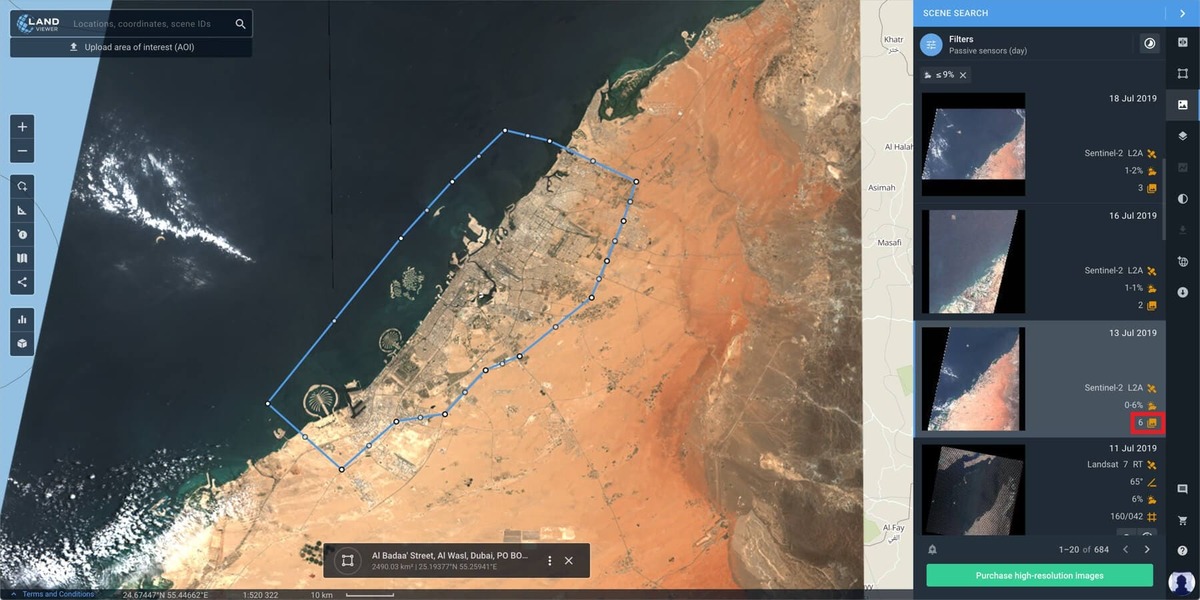
1. At first set (find, upload, draw) your AOI. When done, in the Filters tab select the sensor, set Cloudiness and Sun Elevation values. If your AOI is not covered with a single image, the Mosaic will be automatically created to obtain the full coverage. The Mosaic icon indicating the number of scenes in mosaic is displayed in the image preview card.

2. Once the Mosaic is chosen you can apply various band combinations. Select the required one from the Band Combinations tab and it will be immediately applied to your image.

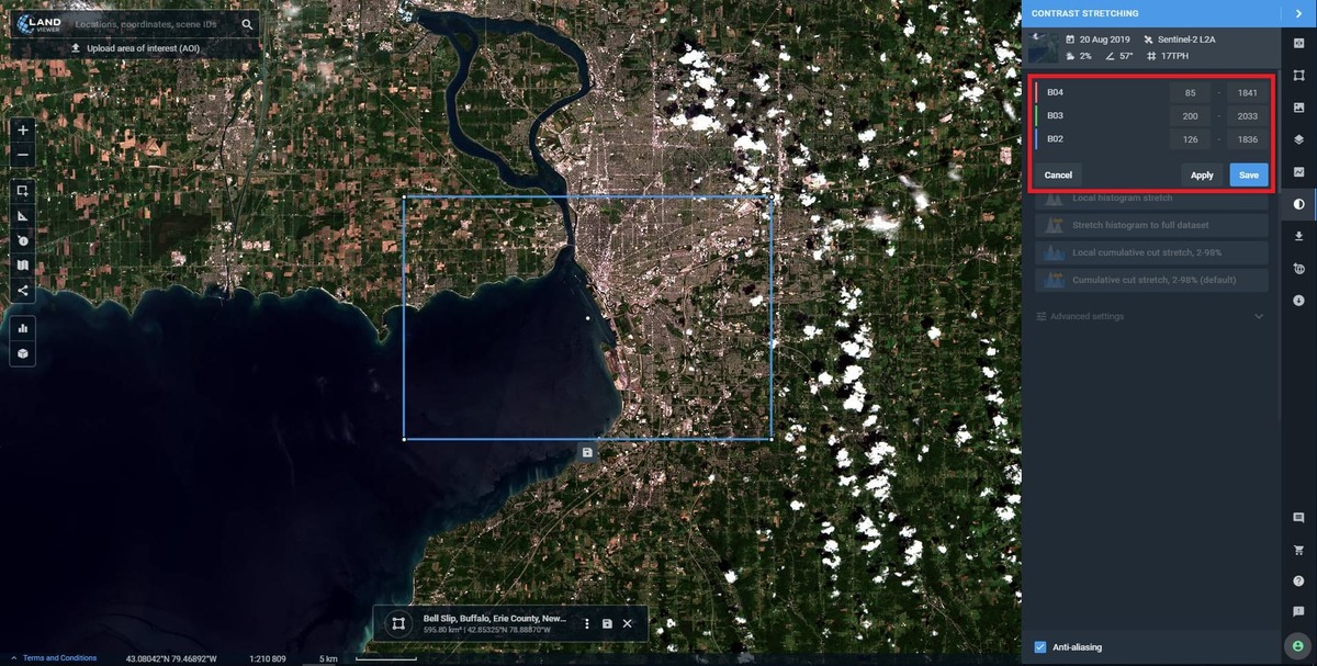
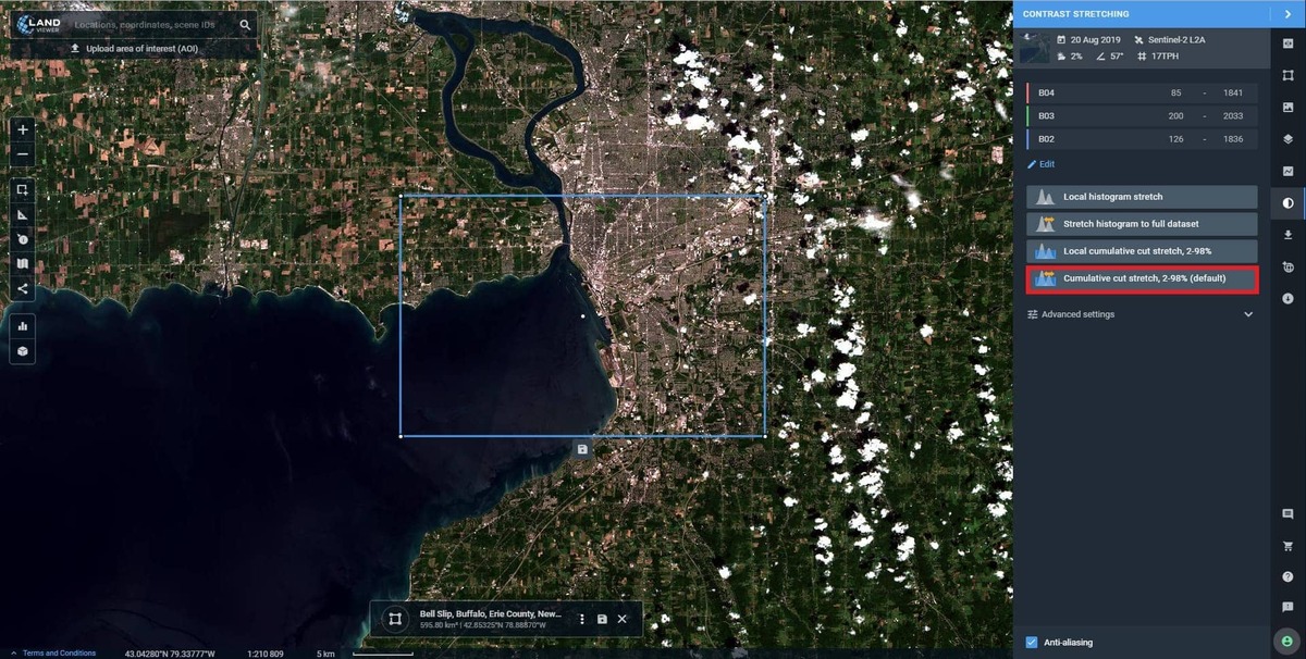
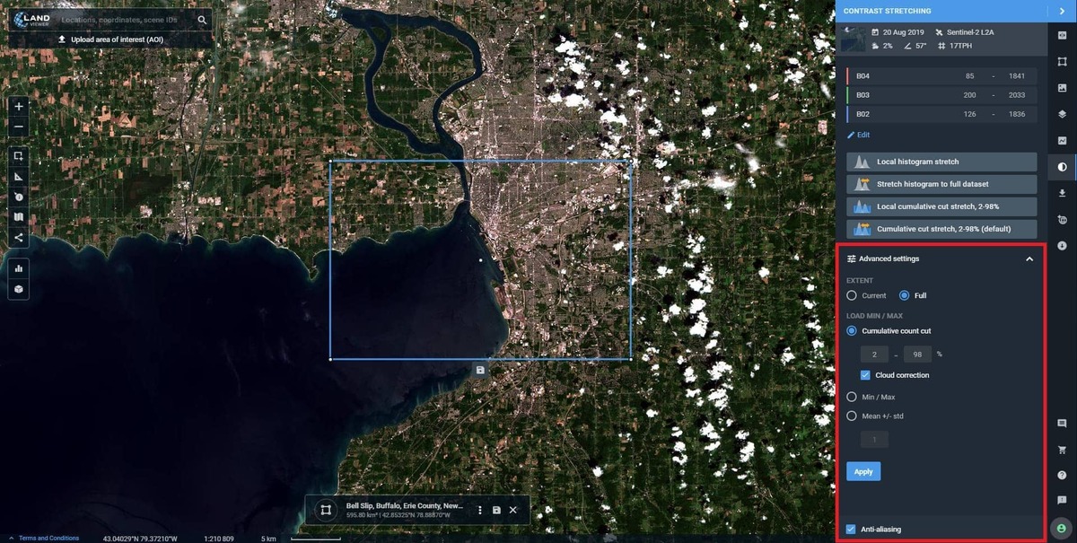
3. There is also a possibility of using Contrast Stretching tool. You can select it from the menu by clicking Contrast stretching tab. Once it’s done hit the Edit button and manually set the required parameters. You can apply changes for previewing and save them when the needed result is achieved.

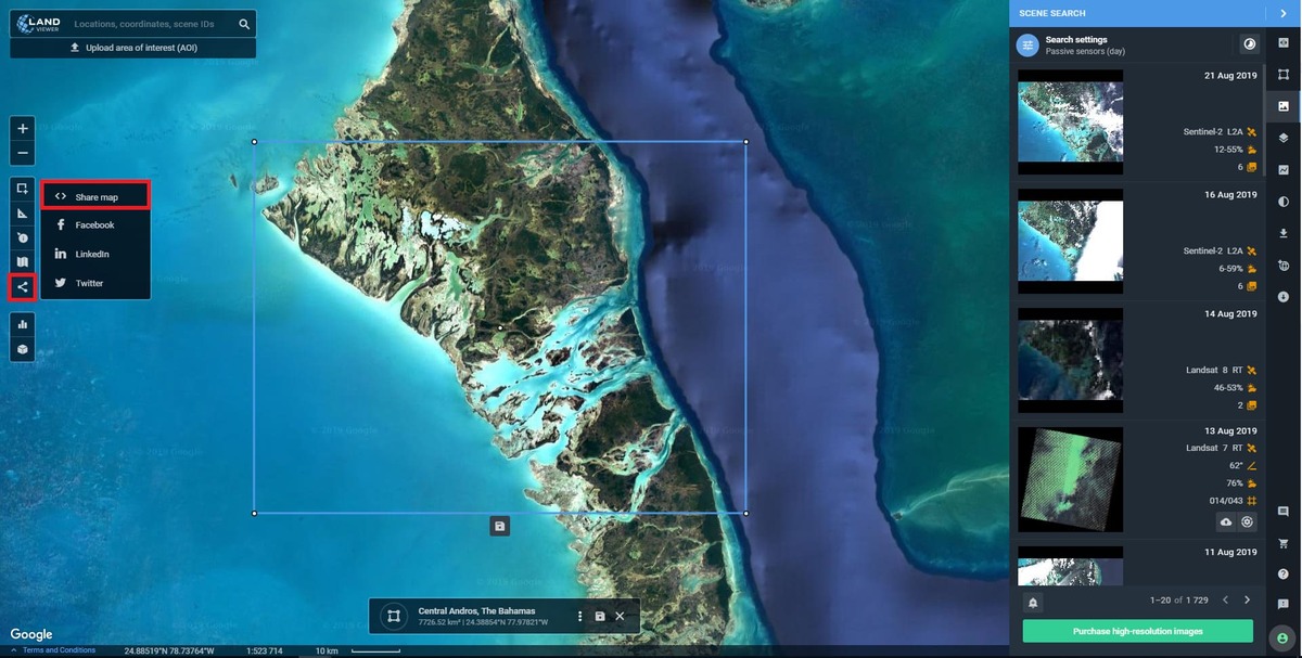
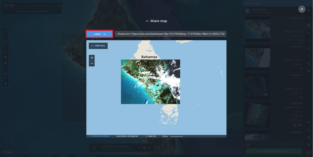
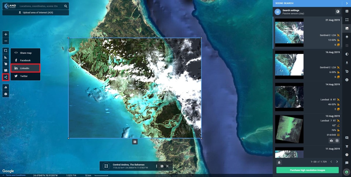
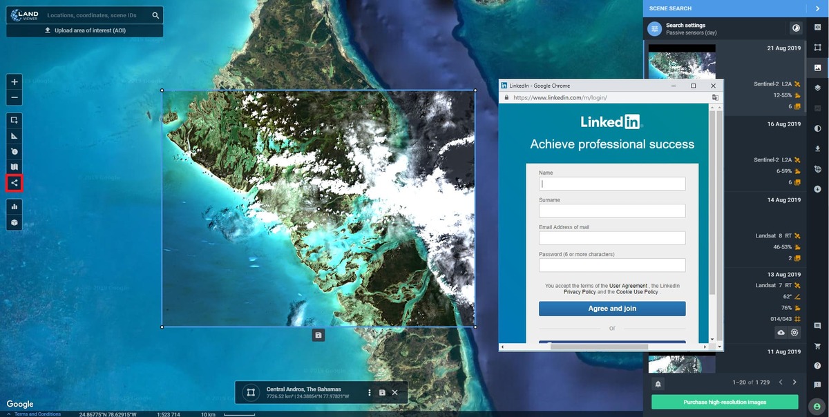
4. You can share your mosaic by clicking the Share button in the tool-box on the left side of the screen. The system offers several sharing options – link creating or sharing via such platforms as Facebook, LinkedIn or Twitter.

Choosing the creation of a link option will lead to an opening of a preview window, with an ability to select file size (small, medium or large).

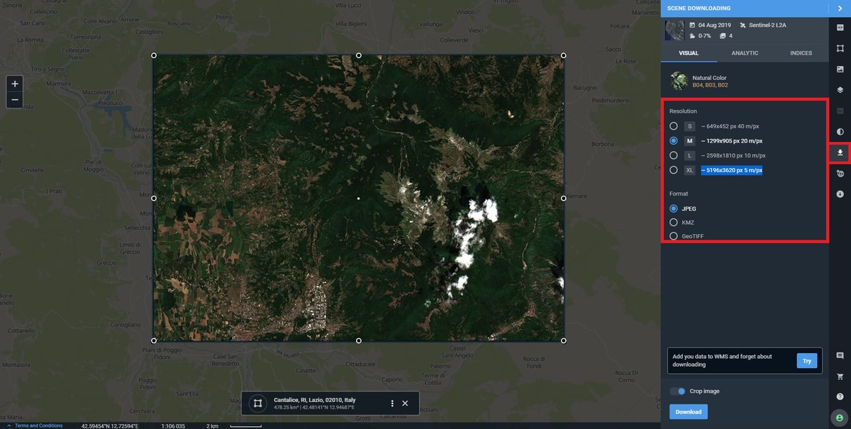
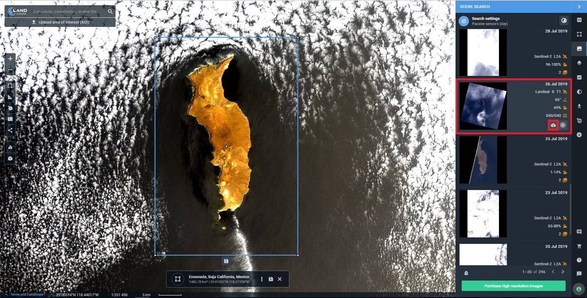
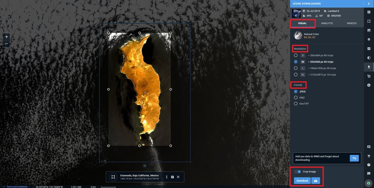
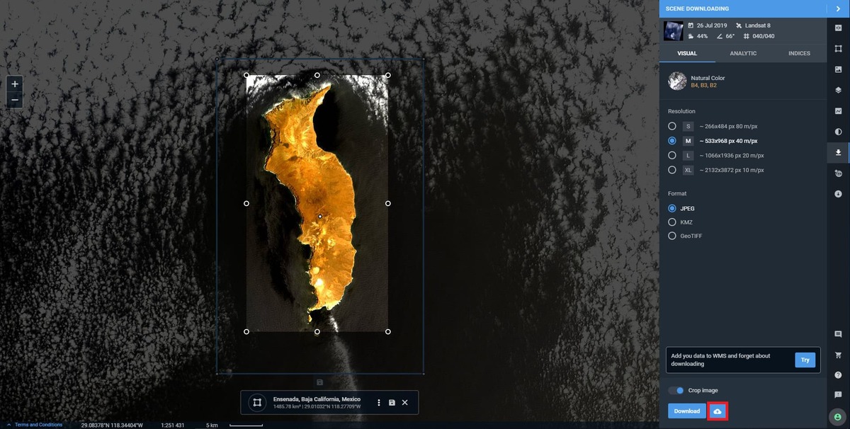
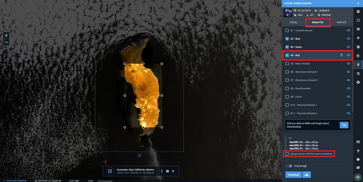
5. To download the Mosaic, go to the Scene Downloading tab. The preview card will appear on the top of the downloading tab. It displays the date, the sensor, cloud coverage, the Sun elevation angle, the number of scenes in the Mosaic. Three types of downloads can be applied to Mosaic, these are  – Visual, Analytics or Indices, depending on the user’s request. 

• In case you select the Visual type, the resulting data will be delivered in the shape of JPEG, KMZ, GeoTIFF file, containing the merged  scenes (e.g. all the scenes that fall into the AOI and don’t intersect.);
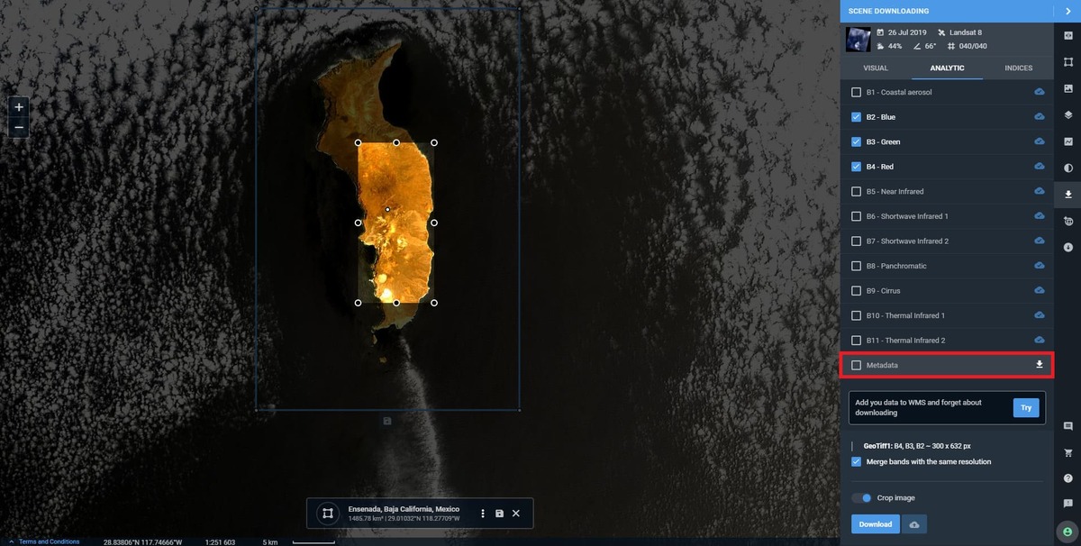
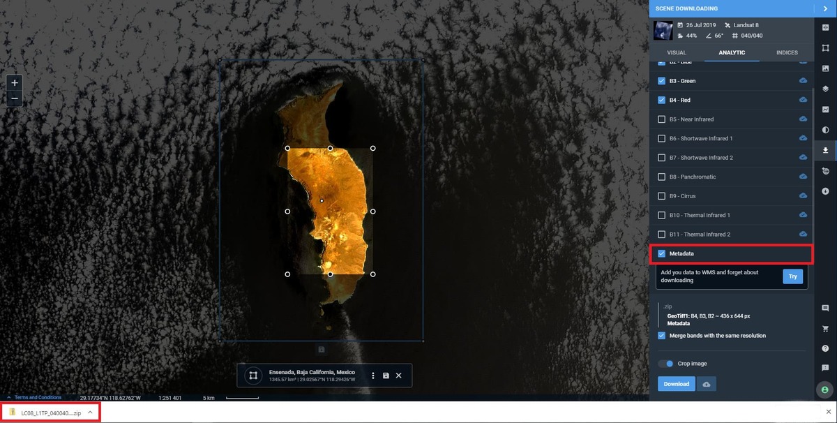
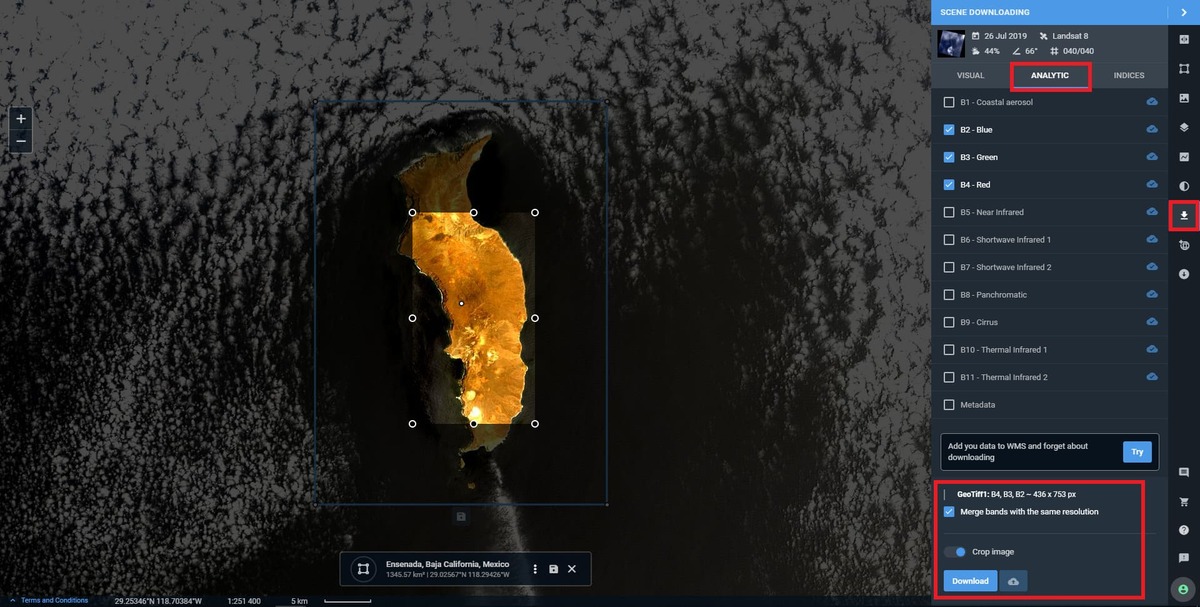
• The download result with the Analytics type will be an archive of the merged bands without metadata, for example (GeoTiff1: B02, GeoTiff2: B03, GeoTiff3: B04, GeoTiff4: B05.);
• With the Indices type, the result data for the mosaic will be presented as a TIFF file.

In the Scene Downloading menu, you can select the resolution of the image and its format. Select one of the suggested resolutions (S ~ 649×452 px 40 m/px, M ~ 1299×905 px 20 m/px, L ~ 2598×1810 px 10 m/px or XL ~ 5196×3620 px 5 m/px) that display ground sampling distance and the most suitable file format (JPEG, KMZ or GeoTIFF).

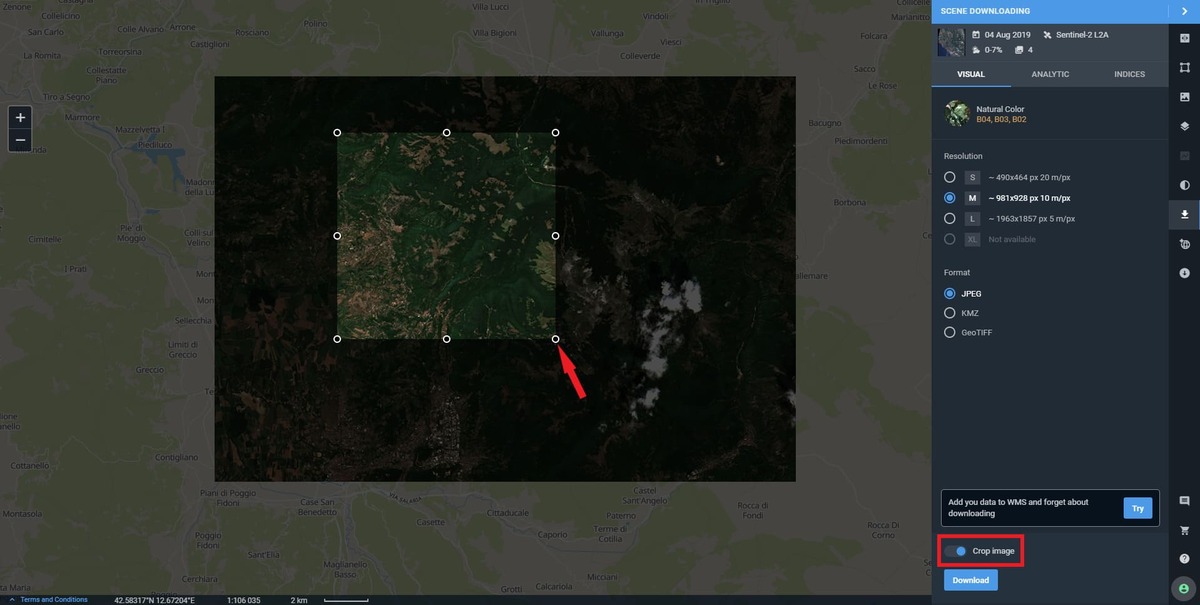
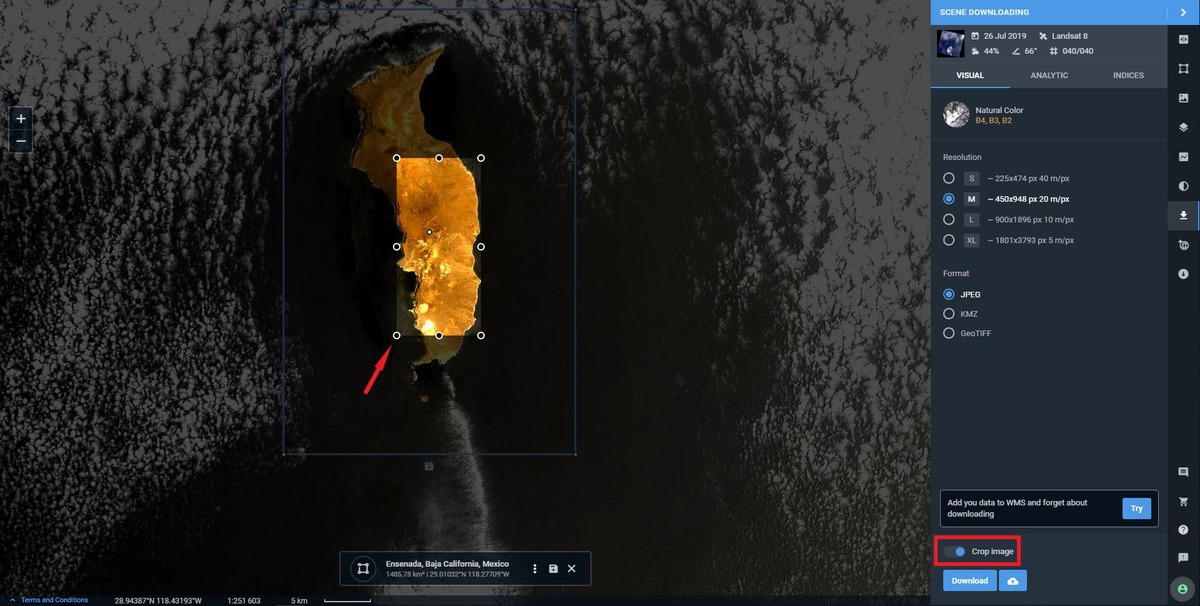
There is also an option to download by crop. To use this function you should enable the Crop image switch at the bottom of the Scene Downloading menu and stretch the bbox to set the area you want to download. In case the crop parameters are not set, all scenes are downloaded fully.

Once you select all needed settings, click the Download button at the bottom of the menu and you will see a pop-up displaying the start of the downloading. Also, please note that if you want to crop beyond the territory, covered by your AOI, the image will nevertheless be saved within the set AOI. The download limit for one file is 2 GB.

Applied fields

Agro monitoring: identify crop yields on a large scale, assess multiple fields all-in-one, no matter what territory they occupy, apply different vegetation indices and build fertilizers for all your fields at once, analyze your territories without data loss – sowing, watering, weather risks as well as farming equipment map.

Natural disasters: assessment of natural and man-made disasters impact. Fire monitoring, identification of droughts, defining of the damaged areas with the help of specific indices on a large territories. Observe floods and detect their sources no matter how far they are.

Coastal monitoring: analysis of coastal zones of long extent, monitoring of coastline changes, bathymetric analysis of water bodies as a whole through comparsion of images from different times, monitor melting of glaciers no matter how big they are, watch out for arctic rivers change.

Construction: monitoring and change detection of construction development within a large area of interest, mostly it comes in use for companies who are going to put in action ambitious projects on a large areas to keep track of which using traditional methods is impossible. This feature will be extremely useful for road designers and constructors. Pave roads guided by the latest up-to-date images composed in a convenient mosaic without any displacements or losses.

Forestry: monitoring of illegal deforestation on a large scale using mosaic approach to assess the damage of such activities.

Change Detection

The objective of Change Detection is to compare the spatial representation of two points in time by controlling all variances caused by differences in variables that are not of interest and to measure changes caused by differences in the variables of interest.  Change detection for GIS  is a process that measures how the attributes of a particular area have changed between two or more time periods, comparing two satellite images taken at different times. Change detection has been widely used to assess deforestation, urban growth, the impact of natural disasters and land cover changes etc.

To get started with the Change Detection function, please follow several simple steps:

1. Firstly set/upload/draw your area of interest (AOI). Once it’s done, in the FILTERS tab select the sensor, set Cloudiness and Sun Elevation values. After that, go to Analysis Tools menu and click Change Detection.

NB You need to select the scene to make the Change Detection active.

2. Once the first image is chosen, it appears on the map in the left side of the Comparison slider, while the right part contains the search panel to find the second image. When you get started with searching, a prompt message on how to proceed in a proper way occurs in the right menu. The Cloudiness is set up to 30% and the data source is chosen accordingly to the first image sensor by default.  Use the buttons L / R to switch between the images on the slider.

3. At this step, please select the second image, dating from a different period of time to detect and assess the changes happened.  Once both images appear on the map, click the Change Detection button to access the feature’s menu.

4. Choose the index you want to detect the changes for from the list in the Indices drop-down menu. To make whatever setting’s changes Click the “Back to scene search” button in the right upper menu. You can also check both images metadata and switch between the images on the map clicking the thumbnail pictures in turn. In order to select the necessary index go to Band combination drop-down menu. The scenes are displayed in “natural color”.

5. Once all the options are set, click Calculate. The outcome image is displayed over the originals ones.  Once it is calculated, a slider to change the transparency of the difference layer appears on the map, and, below you can find the Change Detection Legend, displaying the index values by different colors. In our case, the resulting image shows positive changes in NDVI values.

6. Now you can either download the image in .png, .tiff or .jpeg  format on your device or save it to your EOSDA Storage account.

Time Series Analysis

With Time Series Analysis, you can visualize the data dynamics, constructing a spatiotemporal time series vegetation indices (VI) graph. The approach is widely employed in regional vegetation growth dynamics observation, phenological crop identification, land use change detection, etc. To use the Time Series Analysis is easy.  You just need to set the AOI, time period and vegetation index. Once the graph is built,  check the metric details of the selected Scene, Preview it on the map and download the result data as Excel file for further processing.  

To get started with Time Series Analysis, take the following steps:

• Set the AOI (maximum processing area –  200 km2) and click the Time Series Analysis icon

• Choose the spectral index (NDVI, NDWI, NDSI) from the drop-down menu in the Time Series section on the top of the graph. Then select the sensor from the drop-down menu and time period; time intervals of (1, 3, 6, 12) months and (3, 5, 10) years are set by default. To build analytics with the selected parameters click Apply

• click Figure or Table on the right of the graph to download the result data as CSV file for further processing

• Left-click the point on the graph to check the metric details of the particular Scene, that is Source Data, Cloudiness, Mean, P10/P90, Median, sd, Min / Max

• To Preview the result, click Visualize in the top right of the image and the selected Scene shows up on the map

High resolution imagery (for analytics)

EOSDA LandViewer is connected to Airbus SE via API, therefore you can preview high-res satellite images, select the one that fits your AOI most and purchase it. The procedure is as follows:

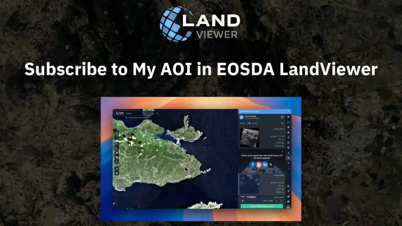
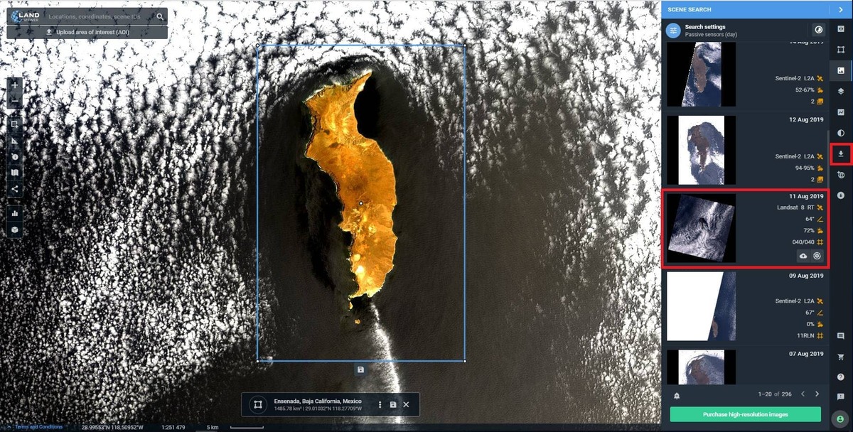
• Set the AOI and select High resolution imagery (for analytics) category in the Source drop-down menu of All Filters tab. Apply the other filters

Preview the available scenes on the map and check the details. The price is given in US dollars and highlighted in green. It also provides you with the information about the area of intersection between the selected image and your AOI the final price is based on. In other words, the larger the area of intersection, the higher the price charged. Select the necessary images and click Add to cart.

Check the adding progress status, which is displayed in the bottom right of the screen. Once the process is completed, the notification In cart shows up in the image field.

Click Your Cart icon to check the order.

In the cart box specify the number of end-users in License field, tick the EULA (End-User License Agreement) box to confirm you agree to terms and click Submit.

NB We also offer a flexible discount system that depends on the number of images as well as the size of the area purchased.

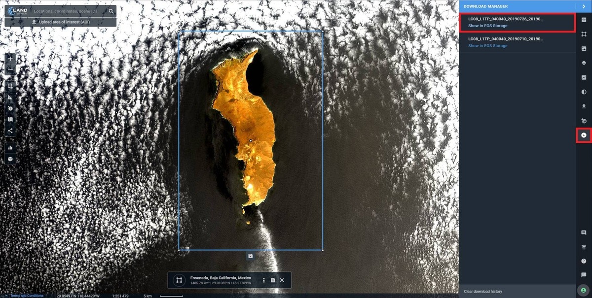
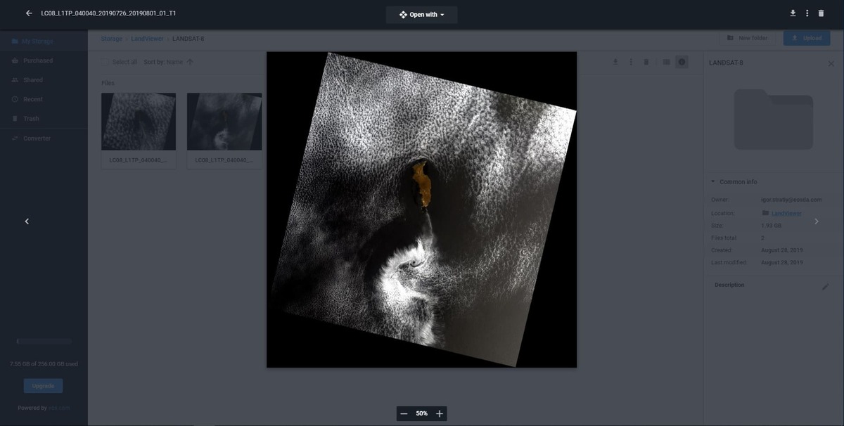
The notification box shows up once your request is successfully sent. Once all the purchased details are agreed, the payment link or invoice shows up in the middle of the screen. When the payment is received, the image is distributed it to your EOSDA Storage account within three business days. At this step, you can download the purchased high-resolution satellite images directly from the EOSDA Storage.

3D Modeling

Create a three-dimensional representation of your AOI with a powerful visualization tool – 3D Terrain Modeling. How to use it:

• set the AOI, select the Terrain layer and click the 3D Modeling icon in the toolbar on the left

• wait a few seconds until 3D Modeling is in progress

• customize your 3D Model, using (+) and (-),  the mouse buttons and keyboard arrows

Zoom in to view the terrain details

To make a 3D Model of the satellite image, set the AOI, select the image and apply 3D Modeling feature

Wait a few seconds until 3D Modeling is in progress and navigate the Model according to your needs

WMS

With WMS (Web Maps Serviсе) you can integrate EOSDA LandViewer data into 3rd party tool. Using the function, browse the imagery from EOSDA LandViewer directly in your desktop or online software applications like QGIS, ArcGIS, EOSDA Vision, etc. for further processing

*To add the data to WMS you should have a client with WMS 1.3 protocol support only

To get started with WMS, take the following steps:

• Set the AOI and click add to WMS layer in the context menu

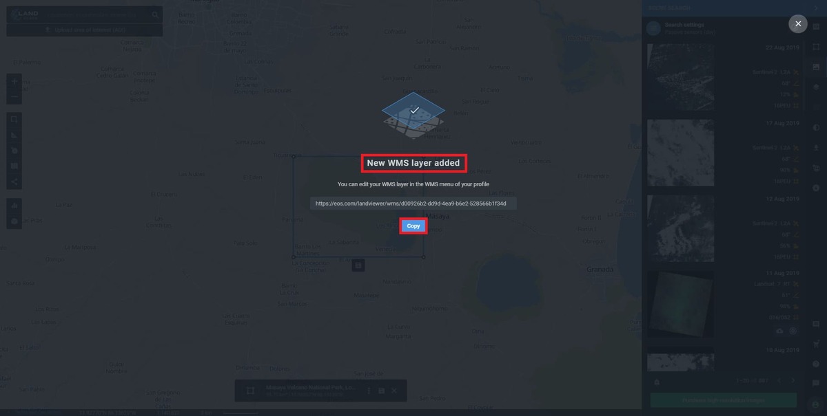
• Once it’s done, in the special WMS box set the Date, check the specifications and click Add to get a wms url link

• Copy it and use for further processing whenever you need

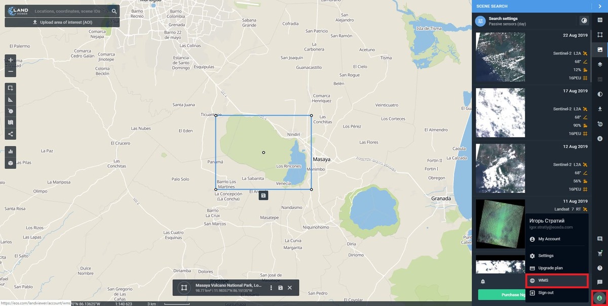
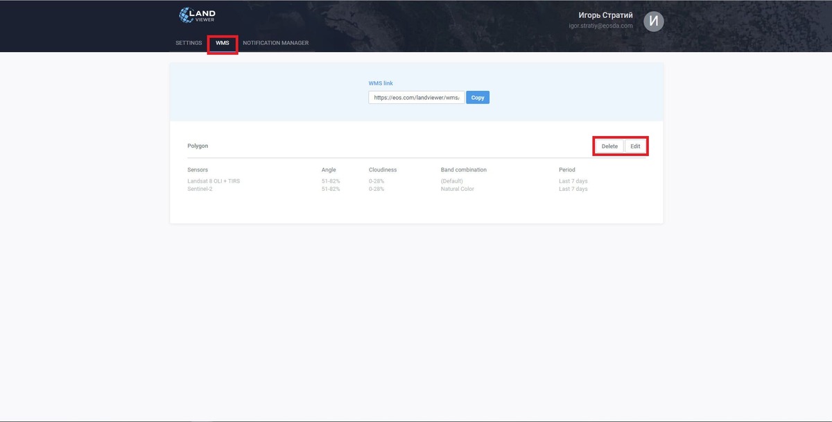
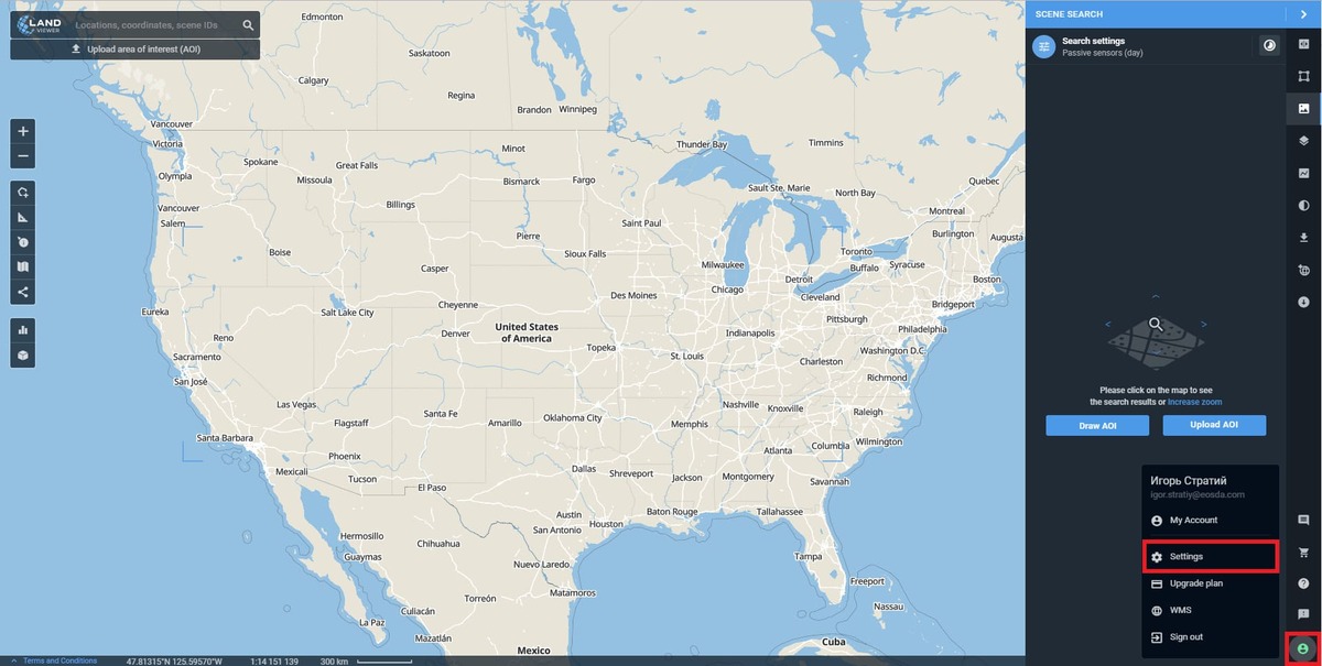
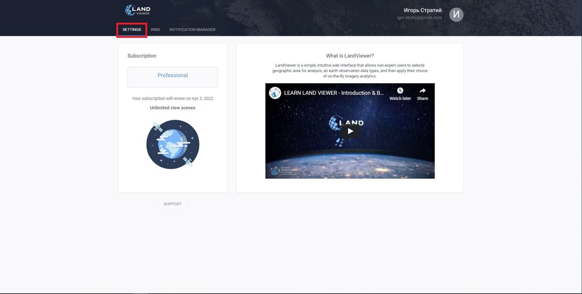
To check, edit and copy the list of your WMS links, stored in the section, go your Profile settings and select WMS

Compare images

To view and compare two images from one or several satellites, use the Comparison slider that splits the screen into two parts. You can also apply the band combinations and spectral indices. To use it:

• set the AOI
• process the image according to your needs
• click Comparison slider in the right sidebar
• once the screen is split into 2 parts (the left part – the processed image, the right one – the base map), repeat the workflow described above.
• move the slider left and right to change the size of the parts

Clustering

Another progressive functionality is designed to specify definite, averaged in definite index ranges, zones within the AOI, with clear boundaries, displaying the results of zone parameters’ calculation and the ability to export them to other software.

How it works

The tool transforms a high-resolution raster map into zones that share common index values. As a result of clustering + vectorization, you will get two new layers within the selected AOI. The first one is a raster layer containing the zones, which are highlighted with respective color and their boundaries determined by the same color. And the other one is vector layer, which contains b/w image, where each particular zone is indicated by a black color outline, and the detailed information about each zone that can be exported directly to a shapefile for further processing in other applications.

1. To get started with Clustering, you should draw your AOI using the tool-box on the left, choose the data source and select the image, covering your AOI 100%.

2. Once it’s done, click Clustering icon on the right

3. Select the Band combination from the drop-down menu, set the number of Classes (zones) and the Minimum zone area you are going to analyze. After that make step 1 and apply Show preview to display the results of raster zone calculation.

4. Make step 2 and click Calculate metrics to start vector calculation. Once the calculation is completed, the results are saved in your EOSDA Storage account by default. To download the layers on your device, click the Download button in the bottom menu.

5. To check the metrics details of the specific zone, left – click any place of the selected zone. Manage color and borders setting using Fills and Borders buttons respectively. Choose the downloading geo-format from the list available.

Applied fields

Agro monitoring: identification of high/low crop yield and affected vegetation areas, different types of vegetation areas to build fertilizers, sowing/resting, watering as well as drones’ routes and farming equipment map.

Coastal monitoring: analysis of coastal zones, coral reefs to assess and analyze water temperature, salinity, phytoplankton, hydrology, changes in coastline, bathymetry, soil moisture as well as potential threats to shores.

Forestry: identification of specific zones by vegetation density, vegetation type, monitoring of deforestation yet together with the vegetation change dynamics using time series approach.

Account settings

Сlick the Account icon and select Settings to find the terms&conditions of your pricing Plan and check new video tutorials. Use the Support button to contact the LV team

My account

To create your account take the following steps:

• In the Profile tab select My Account to get to your Profile page

• Fill in all the required credentials and upload your profile photo

• Go to Security tab to change your password, if needed

• use My activity tab to track your activity (time, action, IP address, location) whenever you need

Feedback

In the main tab select Feedback option to get to the Feedback box

Fill in a special Message form and click Submit to send your feedback, questions or suggestions to LV support team

Sign out

Click Sign out in the Profile tab to exit EOSDA LandViewer

Save to EOSDA Storage

To save the image to EOSDA Storage, select the image for your AOI and click the Download button in the right corner of the image

Click the Scene downloading to check your file in the list

Select the Show in EOSDA Storage option to check your file there

On the EOSDA Storage page select Recent, find the image in the list and right-click it to see all the options available

Extract analytics from the image in EOSDA Processing

Select the image for your AOI and click a gear-wheel icon in the right corner of the image to have it open with EOSDA Processing. Once the processing is completed, the output file is saved to EOSDA Storage by default

Once the file is downloaded, on EOSDA Processing page select the EOSDA LandViewer project from the drop-down menu or Create new project from EOSDA LandViewer processing result

Once the new project is created, hover over the project box to edit, remove or Open Project for further processing

To instantly process and download

Select the image for your AOI, apply all the filters, both the default and custom settings available in EOSDA LandViewer and click Downloading icon in the right-side menu

In the Visual tab select Resolution, Format and use Crop by extent option, if necessary

Click Download button in the bottom right menu to save the image on your device

To save the image to EOSDA Storage click the cloud icon

Download a specific part of the image

Select the required area, use Crop by Extent and click Download button in the bottom of the tab

Download Metadata

Select Metadata in Analytic tab to download extended information on the image (source data, acquisition date, cloudiness, sun elevation, bands, projection parameters and other specifications), which is necessary for image processing in a specialized software, such as ENVI, ERDAS, etc

All the Tile Matadata is downloaded in one file

Download band combinations separately

To Download band combinations separately, go to Analytic tab, hover over the selected band and click downloading icon in the band field. To check the band details click the I – information button.  To download the selected band to EOSDA Storage, use the cloud icon. Don’t forget to clear the Merge bands with the same resolution tick box

Download band combinations as one file

To Download band combinations as one file choose and convert selected bands (BO8, BO4) to GeoTIFF, crop by visible extent on the map. Bands with the same resolution are merged by default, but if you don’t need it, clear the tick box